Electronic antenna
Сайт для тех, кто любит автомобили и не боится гаечных ключей
Антенна Blaupunkt A-R G 01-E
После того, как штатная антенна на Деу Нексия перестала самостоятельно до конца вдвигаться, а при приеме появились весьма раздражающие шумы и треск, и заметно снизилась чувствительность, радио слушать уже не хотелось. Но через какое-то время, когда репертуар на дисках и флешке поднабил оскомину, захотелось послушать и свежие новости, и трепотню ведущих, и даже просто попсы захотелось, я понял, что хорошая автомобильная антенна просто необходима.
В этой статье я опишу проблемы и критерии выбора антенны в автомобиль, а так же пошагово и с фотографиями покажу, как проходила установка автомобильной антенны Blaupunkt A-R G 01-E.
Итак, вначале муки выбора. Хочется, чтобы антенна на авто и ловила хорошо, и стоила не очень дорого, и чтобы выглядела прилично. После N-ного времени, потраченного на размышления и наведение справок в интернете, я понял, что активная внутрисалонная автомобильная антенна будет для меня наиболее оптимальным выбором.
Плюсы: не ржавеет, не изнашивается, не нарушает аэродинамику, не привлекает вандалов и злодеев.
Минусы: требуется питание, чувствительность заметно меняется в зависимости от направления к источнику сигнала и невозможность повторного использования (один раз приклеил- ВСЁ).
Ранее, на ВАЗ 2108, у меня на лобовом стекле была приклеена автомобильная антенна bosch, которая работала в паре с автомагнитолой «Pioneer», чувствительностью и качеством звука я был вполне доволен. Но, как назло, в магазинах «Бош» я не нашел, «Триада» как вариант, мною даже не рассматривалась, и тут на глаза попалась серо-голубая упаковка с надписью «Blaupunkt» стоимостью 800 рублей. Прочитав скудную информацию на коробке и в инструкции, я расплатился на кассе и пошел в другой магазин в этом же здании за инструментом, где при осмотре витрин в самом низу увидел до боли знакомую коробку, такой же расцветки с такими же надписями, только на этикетке было написано 585 рублей. Вспомнив свои права, согласно закона «О защите прав потребителей» я довольно быстро и без выяснения каких-либо отношений сдал свою покупку назад, а в этом магазине, за эту же сумму купил и антенну, и нужную мне торцовую головку.
Установка автомобильной антенны.
Повторюсь еще раз: будем устанавливать внутрисалонную активную антенну «Blaupunkt Fan Line A-R G 01-E.» в автомобиль Дэу Нексия N-100. Но хочу добавить, что установка этой или иной антенны похожей конструкции, допустим, в переднеприводный ВАЗ или другой автомобиль отличаться будет не очень сильно. Так как антенна приклеивается, то, как и у сапера, здесь нет права на ошибку, как в принципе нет и ничего архисложного. Для начала внимательно изучаем инструкцию и рассматриваем комплектность.

Комплект установки
Надо признать, что руководство весьма скудное и на первый взгляд не очень понятное, но вместе мы разберемся. Для начала из упаковочной коробки вырезаем установочный треугольный шаблон по линиям отреза и
Вырезаем шаблон
переходим к автомобилю. Антенну можно установить на лобовое стекло в двух положениях: посредине, в верхней части стекла (усы расположены симметрично) или в правом верхнем углу (усы расположены под углом примерно 90°). В первом варианте чувствительность антенны будет выше, второй больше подходит для города, где важнее избирательность.
С местом установки определились. Я буду ставить вверху посредине. Для того, чтобы после установки антенный кабель был незаметен, его нужно разместить под обивкой потолка. Для этого нужно демонтировать плафон, солнцезащитные козырьки и накладку правой передней стойки крыши.
Снимаем плафон
При помощи небольшой плоской отвертки вынимаем из пазов стекло рассеивателя, а затем, этой же отверткой отгибая защелки, вынимаем из обшивки потолка корпус плафона. Солнцезащитные козырьки и ручка над пассажирской дверью крепятся при помощи саморезов, отворачиваем их крестовой отверткой. Затем снимаем с верхней части проема правой передней двери резиновый уплотнитель, декоративная накладка держится на защелках (чтобы снять начиная сверху тянем за накладку левой рукой, а правой острием отвертки поддеваем возле защелок). Теперь обшивку можно отодвинуть от крыши и прокладывать под ней кабели.
Хорошо очищаем ветровое стекло в месте размещения антенны от загрязнений и жира при помощи моющих средств, влажной салфетки и насухо вытираем чистой тканью.
Приступаем к наклеиванию (не забываем про сапера, и про семь раз отрежь, один отмерь 🙂 ). В вырезанный треугольный шаблон вставляем крышку корпуса, предназначенную для приклеивания к стеклу, выбираем место установки, чтобы вершина треугольника находилась на верхней кромке стекла, а основание было параллельным линии крыши, снимаем защитную пленку, и, плотно прижав к стеклу, приклеиваем. Для того, чтобы полотно антенны «усы» были размещены равномерно, наклеиваем дистанционные шаблоны из комплекта установки (белые полосочки из клейкой бумаги).

Клеим усы
Наклеивать усы начинаем с установки на место (на штифт крышки корпуса) контактной клеммы, затем снимая небольшими участками защитную пленку, ориентируясь по шаблонам, наклеиваем полотно антенны, не касаясь пальцами клеящего слоя. ВАЖНО. Температура поверхности стекла должна быть не ниже 15°С.
Собираем антенну
Ставим корпус на защелки, закрепляем его при помощи меньшего самореза из комплекта установки. Прокладываем вверх к металлу кузова шлейф заземления и закрепляем его при помощи самореза к усилителю крыши, смазав антикоррозионной смазкой из комплекта установки. В моем автомобиле подходящее отверстие было с завода (сверлить не пришлось). Заземление крепить обязательно, без него чувствительность антенны на порядок ниже, а также возможен выход из строя усилителя.
Крепим массовый провод
Далее прокладываем кабель под обшивкой.
Прокладка кабеля
Опускаем вниз по стойке, в нужных местах приклеивая кусочки двустороннего скотча.
Прокладка кабеля 2
Сквозь зазор пропускаем кабель под панель приборов и проводим к месту установки приемника (магнитолы). При прокладке кабеля не допускаем петель, провисаний, сильных натяжений и касаний к острым углам и кромкам. Установку и закрепление снятых деталей проводим в обратном порядке, но лучше это сделать после проверки работы антенны.
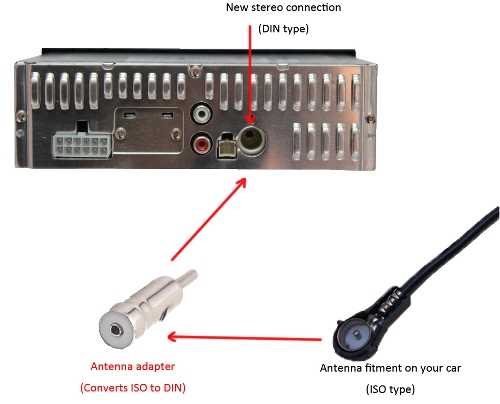
Подключение автомобильной антенны.
На подавляющем большинстве автомобильных проигрывателей производители предусматривают возможность подачи питания для антенны. Распиновку проводов можно посмотреть на наклейке, расположенной на корпусе магнитолы.

Распиновка проводов
В нашем случае это провод голубого цвета, соединяем его с красным проводом питания антенны, а штекер подключаем к гнезду приемника.
Подключаем питание
Я для надежности (электрической и механической) соединения обматываю изолентой. Подключаем разъем к приемнику и проверяем работу. Если все нормально, то на антенне загорится светодиодный индикатор. После этого приклеиваем декоративную накладку.
Вид антенны
Вот так ненавязчиво и стильно антенна выглядит в темноте, кстати подсветку можно отключать при помощи тумблера, расположенного внизу корпуса антенны.
Выкладываю видео. Со старой антенной в этом месте уверенно принималась одна станция, теперь хорошо принимаются шесть, седьмая с треском.

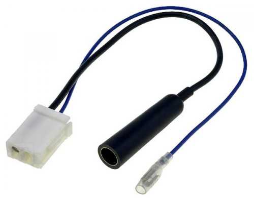
Антенный усилитель
P.S/ Не перестаю удивляться предприимчивости жителей «Поднебесной», создали усилитель радиосигнала который можно инсталлировать в любой автомобиль, буквально за 5 минут ничего не переделывая и превратить любую антенну (штатную, самостоятельно установленную) в активную, или добавить чувствительности той же активной. Как видно по фото штекер усилителя вставляется в гнездо приемника, предназначенное для антенны, антенный штекер в ответную часть усилителя, на синий провод подаем питание +12 v, и можно пробовать. Судя по количеству заказов и и высокому рейтингу отзывов товар явно стоит свои 212 рублей.
Если кто уже пробовал такое устройство поделитесь в комментариях.
УДАЧИ ВАМ НА ДОРОГЕ.
avtomastersam.ru
Antenna (radio)
For other uses, see Antenna.| Part of a series on |
Common types
|
Components
|
Systems
|
Safety and regulation
|
Radiation sources / regions
|
Characteristics
|
Techniques
|
|
| This article needs additional citations for verification. Please help improve this article by adding citations to reliable sources. Unsourced material may be challenged and removed. (January 2014) (Learn how and when to remove this template message) |
In radio and electronics, an antenna (plural antennae or antennas), or aerial, is an electrical device which converts electric power into radio waves, and vice versa.[1] It is usually used with a radio transmitter or radio receiver. In transmission, a radio transmitter supplies an electric current to the antenna's terminals, and the antenna radiates the energy from the current as electromagnetic waves (radio waves). In reception, an antenna intercepts some of the power of an electromagnetic wave in order to produce an electric current at its terminals, that is applied to a receiver to be amplified.
Antennas are essential components of all equipment that uses radio. They are used in systems such as radio broadcasting, broadcast television, two-way radio, communications receivers, radar, cell phones, and satellite communications, as well as other devices such as garage door openers, wireless microphones, Bluetooth-enabled devices, wireless computer networks, baby monitors, and RFID tags on merchandise.
Typically an antenna consists of an arrangement of metallic conductors (elements), electrically connected (often through a transmission line) to the receiver or transmitter. An oscillating current of electrons forced through the antenna by a transmitter will create an oscillating magnetic field around the antenna elements, while the charge of the electrons also creates an oscillating electric field along the elements. These time-varying fields radiate away from the antenna into space as a moving transverse electromagnetic field wave. Conversely, during reception, the oscillating electric and magnetic fields of an incoming radio wave exert force on the electrons in the antenna elements, causing them to move back and forth, creating oscillating currents in the antenna.
Antennas can be designed to transmit and receive radio waves in all horizontal directions equally (omnidirectional antennas), or preferentially in a particular direction (directional or high gain antennas). In the latter case, an antenna may also include additional elements or surfaces with no electrical connection to the transmitter or receiver, such as parasitic elements, parabolic reflectors or horns, which serve to direct the radio waves into a beam or other desired radiation pattern.
The first antennas were built in 1888 by German physicist Heinrich Hertz in his pioneering experiments to prove the existence of electromagnetic waves predicted by the theory of James Clerk Maxwell. Hertz placed dipole antennas at the focal point of parabolic reflectors for both transmitting and receiving. He published his work in Annalen der Physik und Chemie (vol. 36, 1889).
 Animation of a half-wave dipole antenna transmitting radio waves, showing the electric field lines. The antenna in the center is two vertical metal rods, with an alternating current applied at its center from a radio transmitter (not shown). The voltage charges the two sides of the antenna alternately positive (+) and negative (−). Loops of electric field (black lines) leave the antenna and travel away at the speed of light; these are the radio waves. Animated diagram of a half-wave dipole antenna receiving energy from a radio wave. The antenna consists of two metal rods connected to a receiver R. The electric field (E, green arrows) of the incoming wave pushes the electrons in the rods back and forth, charging the ends alternately positive (+) and negative (−). Since the length of the antenna is one half the wavelength of the wave, the oscillating field induces standing waves of voltage (V, represented by red band) and current in the rods. The oscillating currents (black arrows) flow down the transmission line and through the receiver (represented by the resistance R).
 Terminology
Electronic symbol for an antennaThe words antenna (plural: antennas[2] in US English, although both "antennas" and "antennae" are used in International English[3]) and aerial are used interchangeably. Occasionally the term "aerial" is used to mean a wire antenna. However, note the important international technical journal, the IEEE Transactions on Antennas and Propagation.[4] In the United Kingdom and other areas where British English is used, the term aerial is sometimes used although 'antenna' has been universal in professional use for many years.
The origin of the word antenna relative to wireless apparatus is attributed to Italian radio pioneer Guglielmo Marconi. In the summer of 1895, Marconi began testing his wireless system outdoors on his father's estate near Bologna and soon began to experiment with long wire "aerials". Marconi discovered that by raising the "aerial" wire above the ground and connecting the other side of his transmitter to ground, the transmission range was increased.[5] Soon he was able to transmit signals over a hill, a distance of approximately 2.4 kilometres (1.5 mi).[6] In Italian a tent pole is known as l'antenna centrale, and the pole with the wire was simply called l'antenna. Until then wireless radiating transmitting and receiving elements were known simply as aerials or terminals. Because of his prominence, Marconi's use of the word antenna spread among wireless researchers, and later to the general public.[7][8][9]
In common usage, the word antenna may refer broadly to an entire assembly including support structure, enclosure (if any), etc. in addition to the actual functional components. Especially at microwave frequencies, a receiving antenna may include not only the actual electrical antenna but an integrated preamplifier or mixer.
An antenna, in converting radio waves to electrical signals or vice versa, is a form of transducer.[10]
Overview
| This section does not cite any sources. Please help improve this section by adding citations to reliable sources. Unsourced material may be challenged and removed. (January 2014) (Learn how and when to remove this template message) |
Antennas are required by any radio receiver or transmitter to couple its electrical connection to the electromagnetic field. Radio waves are electromagnetic waves which carry signals through the air (or through space) at the speed of light with almost no transmission loss. Radio transmitters and receivers are used to convey signals (information) in systems including broadcast (audio) radio, television, mobile telephones, Wi-Fi (WLAN) data networks, trunk lines and point-to-point communications links (telephone, data networks), satellite links, many remote controlled devices such as garage door openers, and wireless remote sensors, among many others. Radio waves are also used directly for measurements in technologies including radar, GPS, and radio astronomy. In each and every case, the transmitters and receivers involved require antennas, although these are sometimes hidden (such as the antenna inside an AM radio or inside a laptop computer equipped with Wi-Fi).
Whip antenna on car, common example of an omnidirectional antennaAccording to their applications and technology available, antennas generally fall in one of two categories:
- Omnidirectional or only weakly directional antennas which receive or radiate more or less in all directions. These are employed when the relative position of the other station is unknown or arbitrary. They are also used at lower frequencies where a directional antenna would be too large, or simply to cut costs in applications where a directional antenna isn't required.
- Directional or beam antennas which are intended to preferentially radiate or receive in a particular direction or directional pattern.
In common usage "omnidirectional" usually refers to all horizontal directions, typically with reduced performance in the direction of the sky or the ground (a truly isotropic radiator is not even possible). A "directional" antenna usually is intended to maximize its coupling to the electromagnetic field in the direction of the other station, or sometimes to cover a particular sector such as a 120° horizontal fan pattern in the case of a panel antenna at a cell site.
One example of omnidirectional antennas is the very common vertical antenna or whip antenna consisting of a metal rod (often, but not always, a quarter of a wavelength long). A dipole antenna is similar but consists of two such conductors extending in opposite directions, with a total length that is often, but not always, a half of a wavelength long. Dipoles are typically oriented horizontally in which case they are weakly directional: signals are reasonably well radiated toward or received from all directions with the exception of the direction along the conductor itself; this region is called the antenna blind cone or null.
Half-wave dipole antennaBoth the vertical and dipole antennas are simple in construction and relatively inexpensive. The dipole antenna, which is the basis for most antenna designs, is a balanced component, with equal but opposite voltages and currents applied at its two terminals through a balanced transmission line (or to a coaxial transmission line through a so-called balun). The vertical antenna, on the other hand, is a monopole antenna. It is typically connected to the inner conductor of a coaxial transmission line (or a matching network); the shield of the transmission line is connected to ground. In this way, the ground (or any large conductive surface) plays the role of the second conductor of a dipole, thereby forming a complete circuit. Since monopole antennas rely on a conductive ground, a so-called grounding structure may be employed to provide a better ground contact to the earth or which itself acts as a ground plane to perform that function regardless of (or in absence of) an actual contact with the earth.
Diagram of the electric fields (blue) and magnetic fields (red) radiated by a dipole antenna (black rods) during transmission.Antennas more complex than the dipole or vertical designs are usually intended to increase the directivity and consequently the gain of the antenna. This can be accomplished in many different ways leading to a plethora of antenna designs. The vast majority of designs are fed with a balanced line (unlike a monopole antenna) and are based on the dipole antenna with additional components (or elements) which increase its directionality. Antenna "gain" in this instance describes the concentration of radiated power into a particular solid angle of space, as opposed to the spherically uniform radiation of the ideal radiator. The increased power in the desired direction is at the expense of that in the undesired directions. Power is conserved, and there is no net power increase over that delivered from the power source (the transmitter.)
For instance, a phased array consists of two or more simple antennas which are connected together through an electrical network. This often involves a number of parallel dipole antennas with a certain spacing. Depending on the relative phase introduced by the network, the same combination of dipole antennas can operate as a "broadside array" (directional normal to a line connecting the elements) or as an "end-fire array" (directional along the line connecting the elements). Antenna arrays may employ any basic (omnidirectional or weakly directional) antenna type, such as dipole, loop or slot antennas. These elements are often identical.
However a log-periodic dipole array consists of a number of dipole elements of different lengths in order to obtain a somewhat directional antenna having an extremely wide bandwidth: these are frequently used for television reception in fringe areas. The dipole antennas composing it are all considered "active elements" since they are all electrically connected together (and to the transmission line). On the other hand, a superficially similar dipole array, the Yagi-Uda Antenna (or simply "Yagi"), has only one dipole element with an electrical connection; the other so-called parasitic elements interact with the electromagnetic field in order to realize a fairly directional antenna but one which is limited to a rather narrow bandwidth. The Yagi antenna has similar looking parasitic dipole elements but which act differently due to their somewhat different lengths. There may be a number of so-called "directors" in front of the active element in the direction of propagation, and usually a single (but possibly more) "reflector" on the opposite side of the active element.
Greater directionality can be obtained using beam-forming techniques such as a parabolic reflector or a horn. Since high directivity in an antenna depends on it being large compared to the wavelength, narrow beams of this type are more easily achieved at UHF and microwave frequencies.
At low frequencies (such as AM broadcast), arrays of vertical towers are used to achieve directionality [12] and they will occupy large areas of land. For reception, a long Beverage antenna can have significant directivity. For non directional portable use, a short vertical antenna or small loop antenna works well, with the main design challenge being that of impedance matching. With a vertical antenna a loading coil at the base of the antenna may be employed to cancel the reactive component of impedance; small loop antennas are tuned with parallel capacitors for this purpose.
An antenna lead-in is the transmission line (or feed line) which connects the antenna to a transmitter or receiver. The antenna feed may refer to all components connecting the antenna to the transmitter or receiver, such as an impedance matching network in addition to the transmission line. In a so-called aperture antenna, such as a horn or parabolic dish, the "feed" may also refer to a basic antenna inside the entire system (normally at the focus of the parabolic dish or at the throat of a horn) which could be considered the one active element in that antenna system. A microwave antenna may also be fed directly from a waveguide in place of a (conductive) transmission line.
Cell phone base station antennasAn antenna counterpoise or ground plane is a structure of conductive material which improves or substitutes for the ground. It may be connected to or insulated from the natural ground. In a monopole antenna, this aids in the function of the natural ground, particularly where variations (or limitations) of the characteristics of the natural ground interfere with its proper function. Such a structure is normally connected to the return connection of an unbalanced transmission line such as the shield of a coaxial cable.
An electromagnetic wave refractor in some aperture antennas is a component which due to its shape and position functions to selectively delay or advance portions of the electromagnetic wavefront passing through it. The refractor alters the spatial characteristics of the wave on one side relative to the other side. It can, for instance, bring the wave to a focus or alter the wave front in other ways, generally in order to maximize the directivity of the antenna system. This is the radio equivalent of an optical lens.
An antenna coupling network is a passive network (generally a combination of inductive and capacitive circuit elements) used for impedance matching in between the antenna and the transmitter or receiver. This may be used to improve the standing wave ratio in order to minimize losses in the transmission line and to present the transmitter or receiver with a standard resistive impedance that it expects to see for optimum operation.
Reciprocity
It is a fundamental property of antennas that the electrical characteristics of an antenna described in the next section, such as gain, radiation pattern, impedance, bandwidth, resonant frequency and polarization, are the same whether the antenna is transmitting or receiving.[13][14] For example, the "receiving pattern" (sensitivity as a function of direction) of an antenna when used for reception is identical to the radiation pattern of the antenna when it is driven and functions as a radiator. This is a consequence of the reciprocity theorem of electromagnetics.[14] Therefore, in discussions of antenna properties no distinction is usually made between receiving and transmitting terminology, and the antenna can be viewed as either transmitting or receiving, whichever is more convenient.
A necessary condition for the aforementioned reciprocity property is that the materials in the antenna and transmission medium are linear and reciprocal. Reciprocal (or bilateral) means that the material has the same response to an electric current or magnetic field in one direction, as it has to the field or current in the opposite direction. Most materials used in antennas meet these conditions, but some microwave antennas use high-tech components such as isolators and circulators, made of nonreciprocal materials such as ferrite.[13][14] These can be used to give the antenna a different behavior on receiving than it has on transmitting,[13] which can be useful in applications like radar.
Characteristics
| This section needs additional citations for verification. Please help improve this article by adding citations to reliable sources. Unsourced material may be challenged and removed. (January 2014) (Learn how and when to remove this template message) |
Antennas are characterized by a number of performance measures which a user would be concerned with in selecting or designing an antenna for a particular application. Chief among these relate to the directional characteristics (as depicted in the antenna's radiation pattern) and the resulting gain. Even in omnidirectional (or weakly directional) antennas, the gain can often be increased by concentrating more of its power in the horizontal directions, sacrificing power radiated toward the sky and ground. The antenna's power gain (or simply "gain") also takes into account the antenna's efficiency, and is often the primary figure of merit.
Resonant antennas are expected to be used around a particular resonant frequency; an antenna must therefore be built or ordered to match the frequency range of the intended application. A particular antenna design will present a particular feedpoint impedance. While this may affect the choice of an antenna, an antenna's impedance can also be adapted to the desired impedance level of a system using a matching network while maintaining the other characteristics (except for a possible loss of efficiency).
Although these parameters can be measured in principle, such measurements are difficult and require very specialized equipment. Beyond tuning a transmitting antenna using an SWR meter, the typical user will depend on theoretical predictions based on the antenna design or on claims of a vendor.
An antenna transmits and receives radio waves with a particular polarization which can be reoriented by tilting the axis of the antenna in many (but not all) cases. The physical size of an antenna is often a practical issue, particularly at lower frequencies (longer wavelengths). Highly directional antennas need to be significantly larger than the wavelength. Resonant antennas usually use a linear conductor (or element), or pair of such elements, each of which is about a quarter of the wavelength in length (an odd multiple of quarter wavelengths will also be resonant). Antennas that are required to be small compared to the wavelength sacrifice efficiency and cannot be very directional. Fortunately at higher frequencies (UHF, microwaves) trading off performance to obtain a smaller physical size is usually not required.
Resonant antennas
Standing waves on a half wave dipole driven at its resonant frequency. The waves are shown graphically by bars of color (red for voltage, V and blue for current, I) whose width is proportional to the amplitude of the quantity at that point on the antenna.The majority of antenna designs are based on the resonance principle. This relies on the behaviour of moving electrons, which reflect off surfaces where the dielectric constant changes, in a fashion similar to the way light reflects when optical properties change. In these designs, the reflective surface is created by the end of a conductor, normally a thin metal wire or rod, which in the simplest case has a feed point at one end where it is connected to a transmission line. The conductor, or element, is aligned with the electrical field of the desired signal, normally meaning it is perpendicular to the line from the antenna to the source (or receiver in the case of a broadcast antenna).[15]
The radio signal's electrical component induces a voltage in the conductor. This causes an electrical current to begin flowing in the direction of the signal's instantaneous field. When the resulting current reaches the end of the conductor, it reflects, which is equivalent to a 180 degree change in phase. If the conductor is 1⁄4 of a wavelength long, current from the feed point will undergo 90 degree phase change by the time it reaches the end of the conductor, reflect through 180 degrees, and then another 90 degrees as it travels back. That means it has undergone a total 360 degree phase change, returning it to the original signal. The current in the element thus adds to the current being created from the source at that instant. This process creates a standing wave in the conductor, with the maximum current at the feed.[16]
The ordinary half-wave dipole is probably the most widely used antenna design. This consists of two 1⁄4-wavelength elements arranged end-to-end, and lying along essentially the same axis (or collinear), each feeding one side of a two-conductor transmission wire. The physical arrangement of the two elements places them 180 degrees out of phase, which means that at any given instant one of the elements is driving current into the transmission line while the other is pulling it out. The monopole antenna is essentially one half of the half-wave dipole, a single 1⁄4-wavelength element with the other side connected to ground or an equivalent ground plane (or counterpoise). Monopoles, which are one-half the size of a dipole, are common for long-wavelength radio signals where a dipole would be impractically large. Another common design is the folded dipole, which is essentially two dipoles placed side-by-side and connected at their ends to make a single one-wavelength antenna.
The standing wave forms with this desired pattern at the design frequency, f0, and antennas are normally designed to be this size. However, feeding that element with 3f0 (whose wavelength is 1⁄3 that of f0) will also lead to a standing wave pattern. Thus, an antenna element is also resonant when its length is 3⁄4 of a wavelength. This is true for all odd multiples of 1⁄4 wavelength. This allows some flexibility of design in terms of antenna lengths and feed points. Antennas used in such a fashion are known to be harmonically operated.[17]
Current and voltage distribution
The quarter-wave elements imitate a series-resonant electrical element due to the standing wave present along the conductor. At the resonant frequency, the standing wave has a current peak and voltage node (minimum) at the feed. In electrical terms, this means the element has minimum reactance, generating the maximum current for minimum voltage. This is the ideal situation, because it produces the maximum output for the minimum input, producing the highest possible efficiency. Contrary to an ideal (lossless) series-resonant circuit, a finite resistance remains (corresponding to the relatively small voltage at the feed-point) due to the antenna's radiation resistance as well as any actual electrical losses.
Recall that a current will reflect when there are changes in the electrical properties of the material. In order to efficiently send the signal into the transmission line, it is important that the transmission line has the same impedance as the elements, otherwise some of the signal will be reflected back into the antenna. This leads to the concept of impedance matching, the design of the overall system of antenna and transmission line so the impedance is as close as possible, thereby reducing these losses. Impedance matching between antennas and transmission lines is commonly handled through the use of a balun, although other solutions are also used in certain roles. An important measure of this basic concept is the standing wave ratio, which measures the magnitude of the reflected signal.
Consider a half-wave dipole designed to work with signals 1 m wavelength, meaning the antenna would be approximately 50 cm across. If the element has a length-to-diameter ratio of 1000, it will have an inherent resistance of about 63 ohms. Using the appropriate transmission wire or balun, we match that resistance to ensure minimum signal loss. Feeding that antenna with a current of 1 ampere will require 63 volts of RF, and the antenna will radiate 63 watts (ignoring losses) of radio frequency power. Now consider the case when the antenna is fed a signal with a wavelength of 1.25 m; in this case the reflected current would arrive at the feed out-of-phase with the signal, causing the net current to drop while the voltage remains the same. Electrically this appears to be a very high impedance. The antenna and transmission line no longer have the same impedance, and the signal will be reflected back into the antenna, reducing output. This could be addressed by changing the matching system between the antenna and transmission line, but that solution only works well at the new design frequency.
The end result is that the resonant antenna will efficiently feed a signal into the transmission line only when the source signal's frequency is close to that of the design frequency of the antenna, or one of the resonant multiples. This makes resonant antenna designs inherently narrowband, and they are most commonly used with a single target signal. They are particularly common on radar systems, where the same antenna is used for both broadcast and reception, or for radio and television broadcasts, where the antenna is working with a single frequency. They are less commonly used for reception where multiple channels are present, in which case additional modifications are used to increase the bandwidth, or entirely different antenna designs are used.
Electrically short antennas
It is possible to use simple impedance matching concepts to allow the use of monopole or dipole antennas substantially shorter than the ¼ or ½ wavelength, respectively, at which they are resonant. As these antennas are made shorter (for a given frequency) their impedance becomes dominated by a series capacitive (negative) reactance; by adding a series inductance with the opposite (positive) reactance – a so-called loading coil – the antenna's reactance may be cancelled leaving only a pure resistance. Sometimes the resulting (lower) electrical resonant frequency of such a system (antenna plus matching network) is described using the concept of electrical length, so an antenna used at a lower frequency than its resonant frequency is called an electrically short antenna.
For example, at 30 MHz (10 m wavelength) a true resonant ¼ wavelength monopole would be almost 2.5 meters long, and using an antenna only 1.5 meters tall would require the addition of a loading coil. Then it may be said that the coil has lengthened the antenna to achieve an electrical length of 2.5 meters. However, the resulting resistive impedance achieved will be quite a bit lower than that of a true ¼ wave (resonant) monopole, often requiring further impedance matching (a transformer) to the desired transmission line. For ever shorter antennas (requiring greater "electrical lengthening") the radiation resistance plummets (approximately according to the square of the antenna length), so that the mismatch due to a net reactance away from the electrical resonance worsens. Or one could as well say that the equivalent resonant circuit of the antenna system has a higher Q factor and thus a reduced bandwidth, which can even become inadequate for the transmitted signal's spectrum. Resistive losses due to the loading coil, relative to the decreased radiation resistance, entail a reduced electrical efficiency, which can be of great concern for a transmitting antenna, but bandwidth is the major factor[dubious – discuss] that sets the size of antennas at 1 MHz and lower frequencies.
Arrays and reflectors
 Rooftop television Yagi-Uda antennas like these are widely used at VHF and UHF frequencies.
 The amount of signal received from a distant transmission source is essentially geometric in nature due to the inverse-square law, and this leads to the concept of effective area. This measures the performance of an antenna by comparing the amount of power it generates to the amount of power in the original signal, measured in terms of the signal's power density in Watts per square metre. A half-wave dipole has an effective area of 0.13 λ {\displaystyle \lambda } 2. If more performance is needed, one cannot simply make the antenna larger. Although this would intercept more energy from the signal, due to the considerations above, it would decrease the output significantly due to it moving away from the resonant length. In roles where higher performance is needed, designers often use multiple elements combined together.
Returning to the basic concept of current flows in a conductor, consider what happens if a half-wave dipole is not connected to a feed point, but instead shorted out. Electrically this forms a single 1⁄2-wavelength element. But the overall current pattern is the same; the current will be zero at the two ends, and reach a maximum in the center. Thus signals near the design frequency will continue to create a standing wave pattern. Any varying electrical current, like the standing wave in the element, will radiate a signal. In this case, aside from resistive losses in the element, the rebroadcast signal will be significantly similar to the original signal in both magnitude and shape. If this element is placed so its signal reaches the main dipole in-phase, it will reinforce the original signal, and increase the current in the dipole. Elements used in this way are known as passive elements.
A Yagi-Uda array uses passive elements to greatly increase gain. It is built along a support boom that is pointed toward the signal, and thus sees no induced signal and does not contribute to the antenna's operation. The end closer to the source is referred to as the front. Near the rear is a single active element, typically a half-wave dipole or folded dipole. Passive elements are arranged in front (directors) and behind (reflectors) the active element along the boom. The Yagi has the inherent quality that it becomes increasingly directional, and thus has higher gain, as the number of elements increases. However, this also makes it increasingly sensitive to changes in frequency; if the signal frequency changes, not only does the active element receive less energy directly, but all of the passive elements adding to that signal also decrease their output as well and their signals no longer reach the active element in-phase.
It is also possible to use multiple active elements and combine them together with transmission lines to produce a similar system where the phases add up to reinforce the output. The antenna array and very similar reflective array antenna consist of multiple elements, often half-wave dipoles, spaced out on a plane and wired together with transmission lines with specific phase lengths to produce a single in-phase signal at the output. The log-periodic antenna is a more complex design that uses multiple in-line elements similar in appearance to the Yagi-Uda but using transmission lines between the elements to produce the output.
Reflection of the original signal also occurs when it hits an extended conductive surface, in a fashion similar to a mirror. This effect can also be used to increase signal through the use of a reflector, normally placed behind the active element and spaced so the reflected signal reaches the element in-phase. Generally the reflector will remain highly reflective even if it is not solid; gaps less than 1⁄10 λ {\displaystyle \lambda } generally have little effect on the outcome. For this reason, reflectors often take the form of wire meshes or rows of passive elements, which makes them lighter and less subject to wind-load effects, of particular importance when mounted at higher elevations with respect to the surrounding structures. The parabolic reflector is perhaps the best known example of a reflector-based antenna, which has an effective area far greater than the active element alone.
Bandwidth
Although a resonant antenna has a purely resistive feed-point impedance at a particular frequency, many (if not most) applications require using an antenna over a range of frequencies. The frequency range or bandwidth over which an antenna functions well can be very wide (as in a log-periodic antenna) or narrow (in a resonant antenna); outside this range the antenna impedance becomes a poor match to the transmission line and transmitter (or receiver). Also in the case of the Yagi-Uda and other end-fire arrays, use of the antenna well away from its design frequency affects its radiation pattern, reducing its directive gain; the usable bandwidth is then limited regardless of impedance matching.
Except for the latter concern, the resonant frequency of an antenna system can always be altered by adjusting a suitable matching network. This is most efficiently accomplished using a matching network at the site of the antenna, since simply adjusting a matching network at the transmitter (or receiver) would leave the transmission line with a poor standing wave ratio.
Instead, it is often desired to have an antenna whose impedance does not vary so greatly over a certain bandwidth. It turns out that the amount of reactance seen at the terminals of a resonant antenna when the frequency is shifted, say, by 5%, depends very much on the diameter of the conductor used. A long thin wire used as a half-wave dipole (or quarter wave monopole) will have a reactance significantly greater than the resistive impedance it has at resonance, leading to a poor match and generally unacceptable performance. Making the element using a tube of a diameter perhaps 1/50 of its length, however, results in a reactance at this altered frequency which is not so great, and a much less serious mismatch and effect on the antenna's net performance. Thus rather thick tubes are often used for the elements; these also have reduced parasitic resistance (loss).
Rather than just using a thick tube, there are similar techniques used to the same effect such as replacing thin wire elements with cages to simulate a thicker element. This widens the bandwidth of the resonance. On the other hand, it is desired for amateur radio antennas to operate at several bands which are widely separated from each other (but not in between). This can often be accomplished simply by connecting elements resonant at those different frequencies in parallel. Most of the transmitter's power will flow into the resonant element while the others present a high (reactive) impedance, thus drawing little current from the same voltage. Another popular solution uses so-called traps consisting of parallel resonant circuits which are strategically placed in breaks along each antenna element. When used at one particular frequency band the trap presents a very high impedance (parallel resonance) effectively truncating the element at that length, making it a proper resonant antenna. At a lower frequency the trap allows the full length of the element to be employed, albeit with a shifted resonant frequency due to the inclusion of the trap's net reactance at that lower frequency.
The bandwidth characteristics of a resonant antenna element can be characterized according to its Q, just as one uses to characterize the sharpness of an L-C resonant circuit. A common mistake is to assume that there is an advantage in an antenna having a high Q (the so-called "quality factor"). In the context of electronic circuitry a low Q generally signifies greater loss (due to unwanted resistance) in a resonant L-C circuit, and poorer receiver selectivity. However this understanding does not apply to resonant antennas where the resistance involved is the radiation resistance, a desired quantity which removes energy from the resonant element in order to radiate it (the purpose of an antenna, after all!). The Q of an L-C-R circuit is defined as the ratio of the inductor's (or capacitor's) reactance to the resistance, so for a certain radiation resistance (the radiation resistance at resonance does not vary greatly with diameter) the greater reactance off-resonance causes the poorer bandwidth of an antenna employing a very thin conductor. The Q of such a narrowband antenna can be as high as 15. On the other hand, the reactance at the same off-resonant frequency of one using thick elements is much less, consequently resulting in a Q as low as 5. These two antennas may perform equivalently at the resonant frequency, but the second antenna will perform over a bandwidth 3 times as wide as the antenna consisting of a thin conductor.
Antennas for use over much broader frequency ranges are achieved using further techniques. Adjustment of a matching network can, in principle, allow for any antenna to be matched at any frequency. Thus the loop antenna built into most AM broadcast (medium wave) receivers has a very narrow bandwidth, but is tuned using a parallel capacitance which is adjusted according to the receiver tuning. On the other hand, log-periodic antennas are not resonant at any frequency but can be built to attain similar characteristics (including feedpoint impedance) over any frequency range. These are therefore commonly used (in the form of directional log-periodic dipole arrays) as television antennas.
Gain
Main article: Antenna gainGain is a parameter which measures the degree of directivity of the antenna's radiation pattern. A high-gain antenna will radiate most of its power in a particular direction, while a low-gain antenna will radiate over a wider angle. The antenna gain, or power gain of an antenna is defined as the ratio of the intensity (power per unit surface area) I {\displaystyle \scriptstyle I} radiated by the antenna in the direction of its maximum output, at an arbitrary distance, divided by the intensity I iso {\displaystyle \scriptstyle I_{\text{iso}}} radiated at the same distance by a hypothetical isotropic antenna which radiates equal power in all directions. This dimensionless ratio is usually expressed logarithmically in decibels, these units are called "decibels-isotropic" (dBi)
G dBi = 10 log I I iso {\displaystyle G_{\text{dBi}}=10\log {I \over I_{\text{iso}}}\,}A second unit used to measure gain is the ratio of the power radiated by the antenna to the power radiated by a half-wave dipole antenna I dipole {\displaystyle \scriptstyle I_{\text{dipole}}} ; these units are called "decibels-dipole" (dBd)
G dBd = 10 log I I dipole {\displaystyle G_{\text{dBd}}=10\log {I \over I_{\text{dipole}}}\,}Since the gain of a half-wave dipole is 2.15 dBi and the logarithm of a product is additive, the gain in dBi is just 2.15 decibels greater than the gain in dBd
G dBi = G dBd + 2.15 {\displaystyle G_{\text{dBi}}=G_{\text{dBd}}+2.15\,}High-gain antennas have the advantage of longer range and better signal quality, but must be aimed carefully at the other antenna. An example of a high-gain antenna is a parabolic dish such as a satellite television antenna. Low-gain antennas have shorter range, but the orientation of the antenna is relatively unimportant. An example of a low-gain antenna is the whip antenna found on portable radios and cordless phones. Antenna gain should not be confused with amplifier gain, a separate parameter measuring the increase in signal power due to an amplifying device.
Effective area or aperture
Main article: Antenna effective areaThe effective area or effective aperture of a receiving antenna expresses the portion of the power of a passing electromagnetic wave which it delivers to its terminals, expressed in terms of an equivalent area. For instance, if a radio wave passing a given location has a flux of 1 pW / m2 (10−12 watts per square meter) and an antenna has an effective area of 12 m2, then the antenna would deliver 12 pW of RF power to the receiver (30 microvolts rms at 75 ohms). Since the receiving antenna is not equally sensitive to signals received from all directions, the effective area is a function of the direction to the source.
Due to reciprocity (discussed above) the gain of an antenna used for transmitting must be proportional to its effective area when used for receiving. Consider an antenna with no loss, that is, one whose electrical efficiency is 100%. It can be shown that its effective area averaged over all directions must be equal to λ2/4π, the wavelength squared divided by 4π. Gain is defined such that the average gain over all directions for an antenna with 100% electrical efficiency is equal to 1. Therefore, the effective area Aeff in terms of the gain G in a given direction is given by:
A e f f = λ 2 4 π G {\displaystyle A_{\mathrm {eff} }={\lambda ^{2} \over 4\pi }\,G}For an antenna with an efficiency of less than 100%, both the effective area and gain are reduced by that same amount. Therefore, the above relationship between gain and effective area still holds. These are thus two different ways of expressing the same quantity. Aeff is especially convenient when computing the power that would be received by an antenna of a specified gain, as illustrated by the above example.
Radiation pattern
Main article: Radiation pattern Polar plots of the horizontal cross sections of a (virtual) Yagi-Uda-antenna. Outline connects points with 3db field power compared to an ISO emitter.
 The radiation pattern of an antenna is a plot of the relative field strength of the radio waves emitted by the antenna at different angles. It is typically represented by a three-dimensional graph, or polar plots of the horizontal and vertical cross sections. The pattern of an ideal isotropic antenna, which radiates equally in all directions, would look like a sphere. Many nondirectional antennas, such as monopoles and dipoles, emit equal power in all horizontal directions, with the power dropping off at higher and lower angles; this is called an omnidirectional pattern and when plotted looks like a torus or donut.
The radiation of many antennas shows a pattern of maxima or "lobes" at various angles, separated by "nulls", angles where the radiation falls to zero. This is because the radio waves emitted by different parts of the antenna typically interfere, causing maxima at angles where the radio waves arrive at distant points in phase, and zero radiation at other angles where the radio waves arrive out of phase. In a directional antenna designed to project radio waves in a particular direction, the lobe in that direction is designed larger than the others and is called the "main lobe". The other lobes usually represent unwanted radiation and are called "sidelobes". The axis through the main lobe is called the "principal axis" or "boresight axis".
Field regions
Main article: Near and far fieldThe space surrounding an antenna can be divided into three concentric regions: the reactive near-field, the radiating near-field (Fresnel region) and the far-field (Fraunhofer) regions. These regions are useful to identify the field structure in each, although there are no precise boundaries.
The far-field region is are far enough from the antenna to neglect its size and shape. It can be assumed that the electromagnetic wave is purely a radiating plane wave (electric and magnetic fields are in phase and perpendicular to each other and to the direction of propagation). This simplifies the mathematical analysis of the radiated field.
Impedance
As an electro-magnetic wave travels through the different parts of the antenna system (radio, feed line, antenna, free space) it may encounter differences in impedance (E/H, V/I, etc.). At each interface, depending on the impedance match, some fraction of the wave's energy will reflect back to the source,[18] forming a standing wave in the feed line. The ratio of maximum power to minimum power in the wave can be measured and is called the standing wave ratio (SWR). A SWR of 1:1 is ideal. A SWR of 1.5:1 is considered to be marginally acceptable in low power applications where power loss is more critical, although an SWR as high as 6:1 may still be usable with the right equipment. Minimizing impedance differences at each interface (impedance matching) will reduce SWR and maximize power transfer through each part of the antenna system.
Complex impedance of an antenna is related to the electrical length of the antenna at the wavelength in use. The impedance of an antenna can be matched to the feed line and radio by adjusting the impedance of the feed line, using the feed line as an impedance transformer. More commonly, the impedance is adjusted at the load (see below) with an antenna tuner, a balun, a matching transformer, matching networks composed of inductors and capacitors, or matching sections such as the gamma match.
Efficiency
Main article: Antenna efficiencyEfficiency of a transmitting antenna is the ratio of power actually radiated (in all directions) to the power absorbed by the antenna terminals. The power supplied to the antenna terminals which is not radiated is converted into heat. This is usually through loss resistance in the antenna's conductors, but can also be due to dielectric or magnetic core losses in antennas (or antenna systems) using such components. Such loss effectively robs power from the transmitter, requiring a stronger transmitter in order to transmit a signal of a given strength.
For instance, if a transmitter delivers 100 W into an antenna having an efficiency of 80%, then the antenna will radiate 80 W as radio waves and produce 20 W of heat. In order to radiate 100 W of power, one would need to use a transmitter capable of supplying 125 W to the antenna. Note that antenna efficiency is a separate issue from impedance matching, which may also reduce the amount of power radiated using a given transmitter. If an SWR meter reads 150 W of incident power and 50 W of reflected power, that means that 100 W have actually been absorbed by the antenna (ignoring transmission line losses). How much of that power has actually been radiated cannot be directly determined through electrical measurements at (or before) the antenna terminals, but would require (for instance) careful measurement of field strength. Fortunately the loss resistance of antenna conductors such as aluminum rods can be calculated and the efficiency of an antenna using such materials predicted.
However loss resistance will generally affect the feedpoint impedance, adding to its resistive (real) component. That resistance will consist of the sum of the radiation resistance Rr and the loss resistance Rloss. If an rms current I is delivered to the terminals of an antenna, then a power of I2Rr will be radiated and a power of I2Rloss will be lost as heat. Therefore, the efficiency of an antenna is equal to Rr / (Rr + Rloss). Of course only the total resistance Rr + Rloss can be directly measured.
According to reciprocity, the efficiency of an antenna used as a receiving antenna is identical to the efficiency as defined above. The power that an antenna will deliver to a receiver (with a proper impedance match) is reduced by the same amount. In some receiving applications, the very inefficient antennas may have little impact on performance. At low frequencies, for example, atmospheric or man-made noise can mask antenna inefficiency. For example, CCIR Rep. 258-3 indicates man-made noise in a residential setting at 40 MHz is about 28 dB above the thermal noise floor. Consequently, an antenna with a 20 dB loss (due to inefficiency) would have little impact on system noise performance. The loss within the antenna will affect the intended signal and the noise/interference identically, leading to no reduction in signal to noise ratio (SNR).
This is fortunate, since antennas at lower frequencies which are not rather large (a good fraction of a wavelength in size) are inevitably inefficient (due to the small radiation resistance Rr of small antennas). Most AM broadcast radios (except for car radios) take advantage of this principle by including a small loop antenna for reception which has an extremely poor efficiency. Using such an inefficient antenna at this low frequency (530–1650 kHz) thus has little effect on the receiver's net performance, but simply requires greater amplification by the receiver's electronics. Contrast this tiny component to the massive and very tall towers used at AM broadcast stations for transmitting at the very same frequency, where every percentage point of reduced antenna efficiency entails a substantial cost.
The definition of antenna gain or power gain already includes the effect of the antenna's efficiency. Therefore, if one is trying to radiate a signal toward a receiver using a transmitter of a given power, one need only compare the gain of various antennas rather than considering the efficiency as well. This is likewise true for a receiving antenna at very high (especially microwave) frequencies, where the point is to receive a signal which is strong compared to the receiver's noise temperature. However, in the case of a directional antenna used for receiving signals with the intention of rejecting interference from different directions, one is no longer concerned with the antenna efficiency, as discussed above. In this case, rather than quoting the antenna gain, one would be more concerned with the directive gain which does not include the effect of antenna (in)efficiency. The directive gain of an antenna can be computed from the published gain divided by the antenna's efficiency.
Polarization
See also: Polarization (waves) § AntennasThe polarization of an antenna refers to the orientation of the electric field (E-plane) of the radio wave with respect to the Earth's surface and is determined by the physical structure of the antenna and by its orientation; note that this designation is totally distinct from the antenna's directionality. Thus, a simple straight wire antenna will have one polarization when mounted vertically, and a different polarization when mounted horizontally. As a transverse wave, the magnetic field of a radio wave is at right angles to that of the electric field, but by convention, talk of an antenna's "polarization" is understood to refer to the direction of the electric field.
Reflections generally affect polarization. For radio waves, one important reflector is the ionosphere which can change the wave's polarization. Thus for signals received following reflection by the ionosphere (a skywave), a consistent polarization cannot be expected. For line-of-sight communications or ground wave propagation, horizontally or vertically polarized transmissions generally remain in about the same polarization state at the receiving location. Matching the receiving antenna's polarization to that of the transmitter can make a very substantial difference in received signal strength.
Polarization is predictable from an antenna's geometry, although in some cases it is not at all obvious (such as for the quad antenna). An antenna's linear polarization is generally along the direction (as viewed from the receiving location) of the antenna's currents when such a direction can be defined. For instance, a vertical whip antenna or Wi-Fi antenna vertically oriented will transmit and receive in the vertical polarization. Antennas with horizontal elements, such as most rooftop TV antennas in the United States, are horizontally polarized (broadcast TV in the U.S. usually uses horizontal polarization). Even when the antenna system has a vertical orientation, such as an array of horizontal dipole antennas, the polarization is in the horizontal direction corresponding to the current flow. The polarization of a commercial antenna is an essential specification.
Polarization is the sum of the E-plane orientations over time projected onto an imaginary plane perpendicular to the direction of motion of the radio wave. In the most general case, polarization is elliptical, meaning that the polarization of the radio waves varies over time. Two special cases are linear polarization (the ellipse collapses into a line) as discussed above, and circular polarization (in which the two axes of the ellipse are equal). In linear polarization the electric field of the radio wave oscillates back and forth along one direction; this can be affected by the mounting of the antenna but usually the desired direction is either horizontal or vertical polarization. In circular polarization, the electric field (and magnetic field) of the radio wave rotates at the radio frequency circularly around the axis of propagation. Circular or elliptically polarized radio waves are designated as right-handed or left-handed using the "thumb in the direction of the propagation" rule. Note that for circular polarization, optical researchers use the opposite right hand rule from the one used by radio engineers.
It is best for the receiving antenna to match the polarization of the transmitted wave for optimum reception. Intermediate matchings will lose some signal strength, but not as much as a complete mismatch. A circularly polarized antenna can be used to equally well match vertical or horizontal linear polarizations. Transmission from a circularly polarized antenna received by a linearly polarized antenna (or vice versa) entails a 3 dB reduction in signal-to-noise ratio as the received power has thereby been cut in half.
Impedance matching
Main article: Impedance matchingMaximum power transfer requires matching the impedance of an antenna system (as seen looking into the transmission line) to the complex conjugate of the impedance of the receiver or transmitter. In the case of a transmitter, however, the desired matching impedance might not correspond to the dynamic output impedance of the transmitter as analyzed as a source impedance but rather the design value (typically 50 ohms) required for efficient and safe operation of the transmitting circuitry. The intended impedance is normally resistive but a transmitter (and some receivers) may have additional adjustments to cancel a certain amount of reactance in order to "tweak" the match. When a transmission line is used in between the antenna and the transmitter (or receiver) one generally would like an antenna system whose impedance is resistive and near the characteristic impedance of that transmission line in order to minimize the standing wave ratio (SWR) and the increase in transmission line losses it entails, in addition to supplying a good match at the transmitter or receiver itself.
Antenna tuning generally refers to cancellation of any reactance seen at the antenna terminals, leaving only a resistive impedance which might or might not be exactly the desired impedance (that of the transmission line). Although an antenna may be designed to have a purely resistive feedpoint impedance (such as a dipole 97% of a half wavelength long) this might not be exactly true at the frequency that it is eventually used at. In some cases the physical length of the antenna can be "trimmed" to obtain a pure resistance. On the other hand, the addition of a series inductance or parallel capacitance can be used to cancel a residual capacitative or inductive reactance, respectively.
In some cases this is done in a more extreme manner, not simply to cancel a small amount of residual reactance, but to resonate an antenna whose resonance frequency is quite different from the intended frequency of operation. For instance, a "whip antenna" can be made significantly shorter than 1/4 wavelength long, for practical reasons, and then resonated using a so-called loading coil. This physically large inductor at the base of the antenna has an inductive reactance which is the opposite of the capacitative reactance that such a vertical antenna has at the desired operating frequency. The result is a pure resistance seen at feedpoint of the loading coil; unfortunately that resistance is somewhat lower than would be desired to match commercial coax.[citation needed]
So an additional problem beyond canceling the unwanted reactance is of matching the remaining resistive impedance to the characteristic impedance of the transmission line. In principle this can always be done with a transformer, however the turns ratio of a transformer is not adjustable. A general matching network with at least two adjustments can be made to correct both components of impedance. Matching networks using discrete inductors and capacitors will have losses associated with those components, and will have power restrictions when used for transmitting. Avoiding these difficulties, commercial antennas are generally designed with fixed matching elements or feeding strategies to get an approximate match to standard coax, such as 50 or 75 ohms. Antennas based on the dipole (rather than vertical antennas) should include a balun in between the transmission line and antenna element, which may be integrated into any such matching network.
Another extreme case of impedance matching occurs when using a small loop antenna (usually, but not always, for receiving) at a relatively low frequency where it appears almost as a pure inductor. Resonating such an inductor with a capacitor at the frequency of operation not only cancels the reactance but greatly magnifies the very small radiation resistance of such a loop.[citation needed] This is implemented in most AM broadcast receivers, with a small ferrite loop antenna resonated by a capacitor which is varied along with the receiver tuning in order to maintain resonance over the AM broadcast band
Antenna types
Antennas can be classified in various ways. The list below groups together antennas under common operating principles, following the way antennas are classified in many engineering textbooks.[19][20][21]
Isotropic: An isotropic antenna (isotropic radiator) is a hypothetical antenna that radiates equal signal power in all directions. It is a mathematical model that is used as the base of comparison to calculate the gain of real antennas. No real antenna can have an isotropic radiation pattern. However approximately isotropic antennas, constructed with multiple elements, are used in antenna testing.
The first four groups below are usually resonant antennas; when driven at their resonant frequency their elements act as resonators. Waves of current and voltage bounce back and forth between the ends, creating standing waves along the elements.
Dipole
"Rabbit ears" dipole antenna for VHF television receptionThe dipole is the prototypical antenna on which a large class of antennas are based. A basic dipole antenna consists of two conductors (usually metal rods or wires) arranged symmetrically, with one side of the balanced feedline from the transmitter or receiver attached to each.[20][22] The most common type, the half-wave dipole, consists of two resonant elements just under a quarter wavelength long. This antenna radiates maximally in directions perpendicular to the antenna's axis, giving it a small directive gain of 2.15 dBi. Although half-wave dipoles are used alone as omnidirectional antennas, they are also a building block of many other more complicated directional antennas.
Yagi-Uda television antenna for analog channels 2-4, 47-68 MHz- Yagi-Uda – One of the most common directional antennas at HF, VHF, and UHF frequencies. Consists of multiple half wave dipole elements in a line, with a single driven element and multiple parasitic elements which serve to create a uni-directional or beam antenna. These typically have gains between 10–20 dBi depending on the number of elements used, and are very narrowband (with a usable bandwidth of only a few percent) though there are derivative designs which relax this limitation. Used for rooftop television antennas, point-to-point communication links, and long distance shortwave communication using skywave ("skip") reflection from the ionosphere.
- Log-periodic dipole array – Often confused with the Yagi-Uda, this consists of many dipole elements along a boom with gradually increasing lengths, all connected to the transmission line with alternating polarity. It is a directional antenna with a wide bandwidth. This makes it ideal for use as a rooftop television antenna, although its gain is much less than a Yagi of comparable size.
- Turnstile – Two dipole antennas mounted at right angles, fed with a phase difference of 90°. This antenna is unusual in that it radiates in all directions (no nulls in the radiation pattern), with horizontal polarization in directions coplanar with the elements, circular polarization normal to that plane, and elliptical polarization in other directions. Used for receiving signals from satellites, as circular polarization is transmitted by many satellites.
- Corner reflector – A directive antenna with moderate gain of about 8 dBi often used at UHF frequencies. Consists of a dipole mounted in front of two reflective metal screens joined at an angle, usually 90°. Used as a rooftop UHF television antenna and for point-to-point data links.
- Patch (microstrip) – A type of antenna with elements consisting of metal sheets mounted over a ground plane. Similar to dipole with gain of 6–9 dBi. Integrated into surfaces such as aircraft bodies. Their easy fabrication using PCB techniques have made them popular in modern wireless devices. Often combined into arrays.
Monopole
Monopole antennas consist of a single conductor such as a metal rod, mounted over the ground or an artificial conducting surface (a so-called ground plane).[20][23] One side of the feedline from the receiver or transmitter is connected to the conductor, and the other side to ground and/or the artificial ground plane. The monopole is best understood as a dipole antenna in which one conductor is omitted; the radiation is generated as if the second arm of the dipole were present due to the effective image current seen as a reflection of the monopole from the ground. Since all of the equivalent dipole's radiation is concentrated in a half-space, the antenna has twice (3 dB increase of) the gain of a similar dipole, not considering losses in the ground plane.
The most common form is the quarter-wave monopole which is one-quarter of a wavelength long and has a gain of 5.12 dBi when mounted over a ground plane. Monopoles have an omnidirectional radiation pattern, so they are used for broad coverage of an area, and have vertical polarization. The ground waves used for broadcasting at low frequencies must be vertically polarized, so large vertical monopole antennas are used for broadcasting in the MF, LF, and VLF bands. Small monopoles are used as nondirectional antennas on portable radios in the HF, VHF, and UHF bands.
Quarter-wave whip antenna on an FM radio for 88-108 MHz- Whip – Type of antenna used on mobile and portable radios in the VHF and UHF bands such as boom boxes, consists of a flexible rod, often made of telescoping segments.
-
- Rubber Ducky – Most common antenna used on portable two way radios and cordless phones due to its compactness, consists of an electrically short wire helix. The helix adds inductance to cancel the capacitive reactance of the short radiator, making it resonant. Very low gain.
-
- Ground plane – a whip antenna with several rods extending horizontally from base of whip attached to the ground side of the feedline. Since whips are mounted above ground, the horizontal rods form an artificial ground plane under the antenna to increase its gain. Used as base station antennas for land mobile radio systems such as police, ambulance and taxi dispatchers.
- Mast radiator – A radio tower in which the tower structure itself serves as the antenna. Common form of transmitting antenna for AM radio stations and other MF and LF transmitters. At its base the tower is usually, but not necessarily, mounted on a ceramic insulator to isolate it from the ground.
- T and inverted L – Consist of a long horizontal wire suspended between two towers with insulators, with a vertical wire hanging down from it, attached to a feedline to the receiver or transmitter. Used on LF and VLF bands. The vertical wire serves as the radiator. Since at these frequencies the vertical wire is electrically short, much shorter than a quarter wavelength, the horizontal wire(s) serve as a capacitive "hat" to increase the current in the vertical radiator, increasing the gain. Very narrow bandwidth, requires loading coil to tune out any remaining capacitive reactance. Requires low resistance ground (electricity).
- Inverted F – Combines the advantages of the compactness of inverted-L antenna, and the good matching of the F-type antenna. The antenna is grounded at the base and fed at some intermediate point. The position of the feed point determines the antenna impedance. Thus, matching can be achieved without the need for an extraneous matching network.
- Umbrella – Very large wire transmitting antennas used on VLF bands. Consists of a central mast radiator tower attached at the top to multiple wires extending out radially from the mast to ground, like a tent or umbrella, insulated at the ends. Extremely narrow bandwidth, requires large loading coil and low resistance counterpoise ground. Used for long range military communications.
Array
VHF collinear array of folded dipolesArray antennas consist of multiple antennas working as a single antenna. Typically they consist of arrays of identical driven elements, usually dipoles fed in phase, giving increased gain over that of a single dipole.[20][24][25]
- Collinear - Consist of a number of dipoles in a vertical line. It is a high gain omnidirectional antenna, meaning more of the power is radiated in horizontal directions and less into the sky or ground and wasted. Gain of 8 to 10 dBi. Used as base station antennas for land mobile radio systems such as police, fire, ambulance, and taxi dispatchers, and sector antennas for cellular base stations.
- Reflective array - multiple dipoles in a two-dimensional array mounted in front of a flat reflecting screen. Used for radar and UHF television transmitting and receiving antennas.
- Phased array - A high gain antenna used at UHF and microwave frequencies which is electronically steerable. It consists of multiple dipoles in a two-dimensional array, each fed through an electronic phase shifter, with the phase shifters controlled by a computer control system. The beam can be instantly pointed in any direction over a wide angle in front of the antenna. Used for military radar and jamming systems.
- Curtain array - Large directional wire transmitting antenna used at HF by shortwave broadcasting stations. It consists of a vertical rectangular array of wire dipoles suspended in front of a flat reflector screen consisting of a vertical "curtain" of parallel wires, all supported between two metal towers. It radiates a horizontal beam of radio waves into the sky above the horizon, which is reflected by the ionosphere to Earth beyond the horizon
- Batwing or superturnstile - A specialized antenna used in television broadcasting consisting of perpendicular pairs of dipoles with radiators resembling bat wings. Multiple batwing antennas are stacked vertically on a mast to make VHF television broadcast antennas. Omnidirectional radiation pattern with high gain in horizontal directions. The batwing shape gives them wide bandwidth.
- Microstrip - an array of patch antennas on a substrate fed by microstrip feedlines. Microwave antenna that can achieve large gains in compact space. Ease of fabrication by PCB techniques have made them popular in modern wireless devices. Beamwidth and polarization can be actively reconfigurable.
Loop
Loop antenna for transmitting at high frequencies, 2m diameter Separate loop antenna for AM radioLoop antennas consist of a loop (or coil) of wire.[20][26][27] Loops with circumference of a wavelength (or integer multiple of the wavelength) are resonant and act somewhat similarly to the half-wave dipole. However a loop small in comparison to the wavelength, also called a magnetic loop, performs quite differently. This antenna interacts directly with the magnetic field of the radio wave, making it relatively insensitive to nearby electrical noise. However it has a very small radiation resistance, typically much smaller than the loss resistance, making it inefficient and thus undesirable for transmitting. They are used as receiving antennas at low frequencies, and also as direction finding antennas.
Ferrite loopstick antenna from an AM broadcast radio, about 4 in (10 cm) long. The antenna is inductive and, in conjunction with a variable capacitor, forms the tuned circuit at the input stage of the receiver.- Ferrite (loopstick) - These are used as the receiving antenna in most consumer AM radios operating in the medium wave broadcast band (and lower frequencies), a notable exception being car radios. Wire is coiled around a ferrite core which greatly increases the coil's inductance. Radiation pattern is maximum at directions perpendicular to the ferrite rod. The null direction of ferrite core antennas are bi-directional and sharper than the maximal directionality. This often makes the null direction more useful than the maximal directionality because the null direction can be used to reject unwanted signals from interferring stations, sometimes allowing reception from stations with weaker signals than interferring stations.
- Quad - consists of multiple wire loops in a line with one functioning as the driven element, and the others as parasitic elements. Used as a directional antenna on the HF bands for shortwave communication.
Aperture
Dielectric lens antenna used in millimeter wave radio telescopeAperture antennas are the main type of directional antennas used at microwave frequencies and above.[20][28] They consist of a small dipole or loop feed antenna inside a three-dimensional guiding structure large compared to a wavelength, with an aperture to emit the radio waves. Since the antenna structure itself is nonresonant they can be used over a wide frequency range by replacing or tuning the feed antenna.
NASA Cassegrain parabolic spacecraft communication antenna, Australia. Uses X band, 8 – 12 GHz. Extremely high gain ~70 dBi.- Parabolic - The most widely used high gain antenna at microwave frequencies and above. Consists of a dish-shaped metal parabolic reflector with a feed antenna at the focus. It can have some of the highest gains of any antenna type, up to 60 dBi, but the dish must be large compared to a wavelength. Used for radar antennas, point-to-point data links, satellite communication, and radio telescopes
- Horn - Simple antenna with moderate gains of 15 to 25 dBi consists of a flaring metal horn attached to a waveguide. Used for applications such as radar guns, radiometers and as feed antennas for parabolic dishes.
- Slot - Consist of a waveguide with one or more slots cut in it to emit the microwaves. Linear slot antennas emit narrow fan-shaped beams. Used as UHF broadcast antennas and marine radar antennas.
- Dielectric resonator - consists of small ball or puck-shaped piece of dielectric material excited by aperture in waveguide Used at millimeter wave frequencies
Traveling wave
Unlike the above antennas, traveling wave antennas are nonresonant so they have inherently broad bandwidth.[20][29] They are typically wire antennas multiple wavelengths long, through which the voltage and current waves travel in one direction, instead of bouncing back and forth to form standing waves as in resonant antennas. They have linear polarization (except for the helical antenna). Unidirectional traveling wave antennas are terminated by a resistor at one end equal to the antenna's characteristic resistance, to absorb the waves from one direction. This makes them inefficient as transmitting antennas.
A typical random wire antenna for shortwave reception, strung between two buildings.- Random wire - This describes the typical antenna used to receive shortwave radio, consisting of a random length of wire either strung outdoors between supports or indoors in a zigzag pattern along walls, connected to the receiver at one end. Can have complex radiation patterns with several lobes at angles to the wire.
- Beverage - Simplest unidirectional traveling wave antenna. Consists of a straight wire one to several wavelengths long, suspended near the ground, connected to the receiver at one end and terminated by a resistor equal to its characteristic impedance, 400 to 800Ω at the other end. Its radiation pattern has a main lobe at a shallow angle in the sky off the terminated end. It is used for reception of skywaves reflected off the ionosphere in long distance "skip" shortwave communication.
- Rhombic - Consists of four equal wire sections shaped like a rhombus. It is fed by a balanced feedline at one of the acute corners, and the two sides are connected to a resistor equal to the characteristic resistance of the antenna at the other. It has a main lobe in a horizontal direction off the terminated end of the rhombus. Used for skywave communication on shortwave bands.
- Helical (axial mode) - Consists of a wire in the shape of a helix mounted above a reflecting screen. It radiates circularly polarized waves in a beam off the end, with a typical gain of 15 dBi. It is used at VHF and UHF frequencies. Often used for satellite communication, which uses circular polarization because it is insensitive to the relative rotation on the beam axis.
- Leaky wave - Microwave antennas consisting of a waveguide or coaxial cable with a slot or apertures cut in it so it radiates continuously along its length.
Effect of ground
Main article: Multipath propagationGround reflections is one of the common types of multipath.[30][31][32]
The radiation pattern and even the driving point impedance of an antenna can be influenced by the dielectric constant and especially conductivity of nearby objects. For a terrestrial antenna, the ground is usually one such object of importance. The antenna's height above the ground, as well as the electrical properties (permittivity and conductivity) of the ground, can then be important. Also, in the particular case of a monopole antenna, the ground (or an artificial ground plane) serves as the return connection for the antenna current thus having an additional effect, particularly on the impedance seen by the feed line.
When an electromagnetic wave strikes a plane surface such as the ground, part of the wave is transmitted into the ground and part of it is reflected, according to the Fresnel coefficients. If the ground is a very good conductor then almost all of the wave is reflected (180° out of phase), whereas a ground modeled as a (lossy) dielectric can absorb a large amount of the wave's power. The power remaining in the reflected wave, and the phase shift upon reflection, strongly depend on the wave's angle of incidence and polarization. The dielectric constant and conductivity (or simply the complex dielectric constant) is dependent on the soil type and is a function of frequency.
For very low frequencies to high frequencies (<30 MHz), the ground behaves as a lossy dielectric,[33] Thus the ground is characterized both by a conductivity [34] and permittivity (dielectric constant) which can be measured for a given soil (but is influenced by fluctuating moisture levels) or can be estimated from certain maps. At lower frequencies the ground acts mainly as a good conductor, which AM middle wave broadcast (.5 - 1.6 MHz) antennas depend on.
At frequencies between 3 and 30 MHz, a large portion of the energy from a horizontally polarized antenna reflects off the ground, with almost total reflection at the grazing angles important for ground wave propagation. That reflected wave, with its phase reversed, can either cancel or reinforce the direct wave, depending on the antenna height in wavelengths and elevation angle (for a sky wave).
On the other hand, vertically polarized radiation is not well reflected by the ground except at grazing incidence or over very highly conducting surfaces such as sea water.[35] However the grazing angle reflection important for ground wave propagation, using vertical polarization, is in phase with the direct wave, providing a boost of up to 6 db, as is detailed below.
The wave reflected by earth can be considered as emitted by the image antenna.At VHF and above (>30 MHz) the ground becomes a poorer reflector. However it remains a good reflector especially for horizontal polarization and grazing angles of incidence. That is important as these higher frequencies usually depend on horizontal line-of-sight propagation (except for satellite communications), the ground then behaving almost as a mirror.
The net quality of a ground reflection depends on the topography of the surface. When the irregularities of the surface are much smaller than the wavelength, the dominant regime is that of specular reflection, and the receiver sees both the real antenna and an image of the antenna under the ground due to reflection. But if the ground has irregularities not small compared to the wavelength, reflections will not be coherent but shifted by random phases. With shorter wavelengths (higher frequencies), this is generally the case.
Whenever both the receiving or transmitting antenna are placed at significant heights above the ground (relative to the wavelength), waves specularly reflected by the ground will travel a longer distance than direct waves, inducing a phase shift which can sometimes be significant. When a sky wave is launched by such an antenna, that phase shift is always significant unless the antenna is very close to the ground (compared to the wavelength).
| This section does not cite any sources. Please help improve this section by adding citations to reliable sources. Unsourced material may be challenged and removed. (January 2014) (Learn how and when to remove this template message) |
The phase of reflection of electromagnetic waves depends on the polarization of the incident wave. Given the larger refractive index of the ground (typically n=2) compared to air (n=1), the phase of horizontally polarized radiation is reversed upon reflection (a phase shift of π {\displaystyle \scriptstyle {\pi }} radians or 180°). On the other hand, the vertical component of the wave's electric field is reflected at grazing angles of incidence approximately in phase. These phase shifts apply as well to a ground modelled as a good electrical conductor.
The currents in an antenna appear as an image in opposite phase when reflected at grazing angles. This causes a phase reversal for waves emitted by a horizontally polarized antenna (left) but not a vertically polarized antenna (center).This means that a receiving antenna "sees" an image of the antenna but with reversed currents. That current is in the same absolute direction as the actual antenna if the antenna is vertically oriented (and thus vertically polarized) but opposite the actual antenna if the antenna current is horizontal.
The actual antenna which is transmitting the original wave then also may receive a strong signal from its own image from the ground. This will induce an additional current in the antenna element, changing the current at the feedpoint for a given feedpoint voltage. Thus the antenna's impedance, given by the ratio of feedpoint voltage to current, is altered due to the antenna's proximity to the ground. This can be quite a significant effect when the antenna is within a wavelength or two of the ground. But as the antenna height is increased, the reduced power of the reflected wave (due to the inverse square law) allows the antenna to approach its asymptotic feedpoint impedance given by theory. At lower heights, the effect on the antenna's impedance is very sensitive to the exact distance from the ground, as this affects the phase of the reflected wave relative to the currents in the antenna. Changing the antenna's height by a quarter wavelength, then changes the phase of the reflection by 180°, with a completely different effect on the antenna's impedance.
The ground reflection has an important effect on the net far field radiation pattern in the vertical plane, that is, as a function of elevation angle, which is thus different between a vertically and horizontally polarized antenna. Consider an antenna at a height h above the ground, transmitting a wave considered at the elevation angle θ. For a vertically polarized transmission the magnitude of the electric field of the electromagnetic wave produced by the direct ray plus the reflected ray is:
| E V | = 2 | E 0 | | cos ( 2 π h λ sin θ ) | {\displaystyle \textstyle {\left|E_{V}\right|=2\left|E_{0}\right|\,\left|\cos \left({2\pi h \over \lambda }\sin \theta \right)\right|}}Thus the power received can be as high as 4 times that due to the direct wave alone (such as when θ=0), following the square of the cosine. The sign inversion for the reflection of horizontally polarized emission instead results in:
| E H | = 2 | E 0 | | sin ( 2 π h λ sin θ ) | {\displaystyle \textstyle {\left|E_{H}\right|=2\left|E_{0}\right|\,\left|\sin \left({2\pi h \over \lambda }\sin \theta \right)\right|}}where:
- E 0 {\displaystyle \scriptstyle {E_{0}}} is the electrical field that would be received by the direct wave if there were no ground.
- θ is the elevation angle of the wave being considered.
- λ {\displaystyle \scriptstyle {\lambda }} is the wavelength.
- h {\displaystyle \scriptstyle {h}} is the height of the antenna (half the distance between the antenna and its image).
For horizontal propagation between transmitting and receiving antennas situated near the ground reasonably far from each other, the distances traveled by the direct and reflected rays are nearly the same. There is almost no relative phase shift. If the emission is polarized vertically, the two fields (direct and reflected) add and there is maximum of received signal. If the signal is polarized horizontally, the two signals subtract and the received signal is largely cancelled. The vertical plane radiation patterns are shown in the image at right. With vertical polarization there is always a maximum for θ=0, horizontal propagation (left pattern). For horizontal polarization, there is cancellation at that angle. Note that the above formulae and these plots assume the ground as a perfect conductor. These plots of the radiation pattern correspond to a distance between the antenna and its image of 2.5λ. As the antenna height is increased, the number of lobes increases as well.
The difference in the above factors for the case of θ=0 is the reason that most broadcasting (transmissions intended for the public) uses vertical polarization. For receivers near the ground, horizontally polarized transmissions suffer cancellation. For best reception the receiving antennas for these signals are likewise vertically polarized. In some applications where the receiving antenna must work in any position, as in mobile phones, the base station antennas use mixed polarization, such as linear polarization at an angle (with both vertical and horizontal components) or circular polarization.
On the other hand, classical (analog) television transmissions are usually horizontally polarized, because in urban areas buildings can reflect the electromagnetic waves and create ghost images due to multipath propagation. Using horizontal polarization, ghosting is reduced because the amount of reflection of electromagnetic waves in the p polarization (horizontal polarization off the side of a building) is generally less than s (vertical, in this case) polarization. Vertically polarized analog television has nevertheless been used in some rural areas. In digital terrestrial television such reflections are less problematic, due to robustness of binary transmissions and error correction.
Mutual impedance and interaction between antennas
Current circulating in one antenna generally induces a voltage across the feedpoint of nearby antennas or antenna elements. The mathematics presented below are useful in analyzing the electrical behaviour of antenna arrays, where the properties of the individual array elements (such as half wave dipoles) are already known. If those elements were widely separated and driven in a certain amplitude and phase, then each would act independently as that element is known to. However, because of the mutual interaction between their electric and magnetic fields due to proximity, the currents in each element are not simply a function of the applied voltage (according to its driving point impedance), but depend on the currents in the other nearby elements. Note that this now is a near field phenomenon which could not be properly accounted for using the Friis transmission equation for instance. This near field effect creates a different set of currents at the antenna terminals resulting in distortions in the far field radiation patterns; however, the distortions may be removed using a simple set of network equations.[36]
The elements' feedpoint currents and voltages can be related to each other using the concept of mutual impedance Z j i {\displaystyle \scriptstyle {Z_{ji}}} between every pair of antennas just as the mutual impedance j ω M {\displaystyle \scriptstyle {j\omega M}} describes the voltage induced in one inductor by a current through a nearby coil coupled to it through a mutual inductance M. The mutual impedance Z 21 {\displaystyle \scriptstyle {Z_{21}}} between two antennas is defined[37] as:
Z j i = v j i i {\displaystyle Z_{ji}={v_{j} \over i_{i}}}where i i {\displaystyle \textstyle {i_{i}}} is the current flowing in antenna i and v j {\displaystyle \textstyle {v_{j}}} is the voltage induced at the open-circuited feedpoint of antenna j due to i 1 {\displaystyle \textstyle {i_{1}}} when all other currents ik are zero. The mutual impendances can be viewed as the elements of a symmetric square impedance matrix Z. Note that the diagonal elements, Z i i = v i i i {\displaystyle Z_{ii}={v_{i} \over i_{i}}} , are simply the driving point impedances of each element.
Using this definition, the voltages present at the feedpoints of a set of coupled antennas can be expressed as the multiplication of the impedance matrix times the vector of currents. Written out as discrete equations, that means:
v 1 = i 1 Z 11 + i 2 Z 12 + ⋯ + i n Z 1 n v 2 = i 1 Z 21 + i 2 Z 22 + ⋯ + i n Z 2 n ⋮ ⋮ ⋮ ⋮ v n = i 1 Z n 1 + i 2 Z n 2 + ⋯ + i n Z n n {\displaystyle {\begin{matrix}v_{1}&=&i_{1}Z_{11}&+&i_{2}Z_{12}&+&\cdots &+&i_{n}Z_{1n}\\v_{2}&=&i_{1}Z_{21}&+&i_{2}Z_{22}&+&\cdots &+&i_{n}Z_{2n}\\\vdots &&\vdots &&\vdots &&&&\vdots \\v_{n}&=&i_{1}Z_{n1}&+&i_{2}Z_{n2}&+&\cdots &+&i_{n}Z_{nn}\end{matrix}}}where:
- v i {\displaystyle \scriptstyle {v_{i}}} is the voltage at the terminals of antenna i {\displaystyle i}
- i i {\displaystyle \scriptstyle {i_{i}}} is the current flowing between the terminals of antenna i {\displaystyle i}
- Z i i {\displaystyle \scriptstyle {Z_{ii}}} is the driving point impedance of antenna i {\displaystyle i}
- Z i j {\displaystyle \scriptstyle {Z_{ij}}} is the mutual impedance between antennas i {\displaystyle i} and j {\displaystyle j} .
 Mutual impedance between parallel λ 2 {\displaystyle \scriptstyle {\lambda \over 2}} dipoles not staggered. Curves Re and Im are the resistive and reactive parts of the impedance.
 As is the case for mutual inductances,
Z i j = Z j i . {\displaystyle \scriptstyle {Z_{ij}\,=\,Z_{ji}}.}This is a consequence of Lorentz reciprocity. For an antenna element i {\displaystyle i} not connected to anything (open circuited) one can write i i = 0 {\displaystyle i_{i}=0} . But for an element i {\displaystyle i} which is short circuited, a current is generated across that short but no voltage is allowed, so the corresponding v i = 0 {\displaystyle \textstyle {v_{i}}=0} . This is the case, for instance, with the so-called parasitic elements of a Yagi-Uda antenna where the solid rod can be viewed as a dipole antenna shorted across its feedpoint. Parasitic elements are unpowered elements that absorb and reradiate RF energy according to the induced current calculated using such a system of equations.
With a particular geometry, it is possible for the mutual impedance between nearby antennas to be zero. This is the case, for instance, between the crossed dipoles used in the turnstile antenna.
Image gallery
Antennas and supporting structures
-
A building rooftop supporting numerous dish and sectored mobile telecommunications antennas (Doncaster, Victoria, Australia).
-
A water tower in Palmerston, Northern Territory with radio broadcasting and communications antennas.
-
A three-sector telephone site in Mexico City.
-
Telephone site concealed as a palm tree.
Diagrams as part of a system
-
Antennas may be connected through a multiplexing arrangement in some applications like this trunked two-way radio example.
-
Antenna network for an emergency medical services base station.
See also
| Wikimedia Commons has media related to Antennas. |
- Radio portal
- Category:Radio frequency antenna types
- Category:Radio frequency propagation
- Cellular repeater
- DXing
- Electromagnetism
- Mobile broadband modem
- Numerical Electromagnetics Code
- Radial (radio)
- Radio masts and towers
- RF connector
- Smart antenna
- TETRA
- Shortwave broadband antenna
References
- ^ Graf, Rudolf F. (1999). Modern Dictionary of Electronics. Newnes. p. 29. ISBN 0750698667.
- ^ In the context of electrical engineering and physics, the plural of antenna is antennas, and it has been this way since about 1950 (or earlier), when a cornerstone textbook in this field, Antennas, was published by the physicist and electrical engineer John D. Kraus of The Ohio State University. Besides in the title, Dr. Kraus noted this in a footnote on the first page of his book. Insects may have "antennae", but this form is not used in the context of electronics or physics.
- ^ For example http://www.telegraph.co.uk/science/science-news/7810454/British-scientists-launch-major-radio-telescope.html; http://www.ic.gc.ca/eic/site/smt-gst.nsf/eng/sf09377.html; "Archived copy". Archived from the original on 2013-10-20. Retrieved 2013-10-19.
- ^ "IEEE Transactions on Antennas and Propagation".
- ^ Marconi, "Wireless Telegraphic Communication: Nobel Lecture, 11 December 1909." Nobel Lectures. Physics 1901–1921. Amsterdam: Elsevier Publishing Company, 1967: 196–222. p. 206.
- ^ "The Nobel Prize in Physics 1909".
- ^ Slyusar, Vadym (20–23 September 2011). "To history of radio engineering’s term "antenna"" (PDF). VIII International Conference on Antenna Theory and Techniques (ICATT’11). Kyiv, Ukraine. pp. 83–85.
- ^ Slyusar, Vadym (21–24 February 2012). "An Italian period on the history of radio engineering’s term "antenna"" (PDF). 11th International Conference Modern Problems of Radio Engineering, Telecommunications and Computer Science (TCSET’2012). Lviv-Slavske, Ukraine. p. 174.
- ^ Slyusar, Vadym (June 2011). "Антенна: история радиотехнического термина" [The Antenna: A History of Radio Engineering’s Term] (PDF). ПЕРВАЯ МИЛЯ Last mile: Electronics: Science, Technology, Business (in Russian). ? (6): 52–64.
- ^ Schantz, Hans Gregory (2003), "Introduction to ultra-wideband antennas" (PDF), Proceedings of the 2003 IEEE UWBST Conference.
- ^ "Media Advisory: Apply Now to Attend the ALMA Observatory Inauguration". ESO Announcement. Retrieved 4 December 2012.
- ^ Carl Smith (1969). Standard Broadcast Antenna Systems, p. 2-1212. Cleveland, Ohio: Smith Electronics, Inc.
- ^ a b c Lonngren, Karl Erik; Savov, Sava V.; Jost, Randy J. (2007). Fundamentals of Electomagnetics With Matlab, 2nd Ed. SciTech Publishing. p. 451. ISBN 1891121588.
- ^ a b c Stutzman, Warren L.; Thiele, Gary A. (2012). Antenna Theory and Design, 3rd Ed. John Wiley & Sons. pp. 560–564. ISBN 0470576642.
- ^ Hall, Gerald (1991). The ARRL Antenna Book (15th edition). ARRL. p. 24. ISBN 0-87259-206-5.
- ^ Hall 1991, p. 25.
- ^ Hall 1991, pp. 31-32.
- ^ Impedance is caused by the same physics as refractive index in optics, although impedance effects are typically one-dimensional, where effects of refractive index is three-dimensional.
- ^ Bevelaqua, Peter J. "Types of Antennas". Antenna Theory. Antenna-theory.com Peter Bevelaqua's private website. Retrieved June 28, 2015.
- ^ a b c d e f g Aksoy, Serkan (2008). "Antennas" (PDF). Lecture Notes-v.1.3.4. Electrical Engineering Dept., Gebze Technical University, Gebze, Turkey. Archived from the original (PDF) on February 22, 2016. Retrieved June 29, 2015.
- ^ Balanis, Constantine A. (2005). Antenna Theory: Analysis and Design. 1 (3rd ed.). John Wiley and Sons. p. 4. ISBN 047166782X.
- ^ Bevelaqua, Dipole Antenna, Antenna-Theory.com
- ^ Bevelaqua, Monopole Antenna, Antenna-Theory.com
- ^ Bevelaqua, Antenna Arrays, Antenna-Theory.com
- ^ Balanis 2005, pp. 283–371
- ^ Bevelaqua, Loop Antennas, Antenna-Theory.com
- ^ Balanis 2005, pp. 231–275
- ^ Balanis 2005, pp. 653–728
- ^ Balanis 2005, pp. 549–602
- ^ Fixed Broadband Wireless System Design, p. 130, at Google Books
- ^ Monopole Antennas, p. 340, at Google Books
- ^ Wireless and Mobile Communication, p. 37, at Google Books
- ^ Silver, H. Ward, ed. (2011). ARRL Antenna Book. Newington, Connecticut: American Radio Relay League. p. 3-2. ISBN 978-0-87259-694-8.
- ^ http://www.fcc.gov/encyclopedia/m3-map-effective-ground-conductivity-united-states-wall-sized-map-am-broadcast-stations
- ^ Silver 2011, p. 3-23
- ^ Chakravorty, Pragnan; Mandal, Durbadal (2016). "Radiation Pattern Correction in Mutually Coupled Antenna Arrays Using Parametric Assimilation Technique". IEEE Transactions on Antennas and Propagation. PP (99): 1–1. ISSN 0018-926X. doi:10.1109/TAP.2016.2578307.
- ^ Kai Fong Lee (1984). Principles of Antenna Theory. John Wiley and Sons Ltd. ISBN 0-471-90167-9.
Further reading
General
- Antenna Theory (3rd edition), by C. Balanis, Wiley, 2005, ISBN 0-471-66782-X;
- Antenna Theory and Design (2nd edition), by W. Stutzman and G. Thiele, Wiley, 1997, ISBN 0-471-02590-9;
- Antennas (4th edition), by J. Kraus and R. Marhefka, McGraw-Hill, 2001, ISBN 0-07-232103-2;
- Antennenbuch, by Karl Rothammel, publ. Franck'sche Verlagshandlung Stuttgart, 1991, ISBN 3-440-05853-0; other editions (in German)
- Antennas for portable Devices, Zhi Ning Chen (edited), John Wiley & Sons in March 2007
- Broadband Planar Antennas: Design and Applications, Zhi Ning Chen and M. Y. W. Chia, John Wiley & Sons in February 2006
Practical design
- Antenna Theory antenna-theory.com
- Antennas Antenna types
- Patch Antenna: From Simulation to Realization EM Talk
- Why Antennas Radiate, Stuart G. Downs, WY6EE (PDF)
- Understanding electromagnetic fields and antenna radiation takes (almost) no math, Ron Schmitt, EDN Magazine, March 2 2000 (PDF)
- Antennas: Generalities, Principle of operation, As electronic component, Hertz Marconi and Other types Antennas etc etc
Theory and simulations
- AN-SOF, "Antenna Simulation Software". Program system for the modeling of antennas and scatterers.
- EM Talk, "Microstrip Patch Antenna", (Theory and simulation of microstrip patch antenna)
- "[1]" Formulas for simulating and optimizing Antenna specs and placement
- "Microwave Antenna Design Calculator" Provides quick estimation of antenna size required for a given gain and frequency. 3 dB and 10 dB beamwidths are also derived; the calculator additionally gives the far-field range required for a given antenna.
- Sophocles J. Orfanidis, "Electromagnetic Waves and Antennas", Rutgers University (20 PDF Chaps. Basic theory, definitions and reference)
- Hans Lohninger, "Learning by Simulations: Physics: Coupled Radiators". vias.org, 2005. (ed. Interactive simulation of two coupled antennas)
- NEC Lab - NEC Lab is a tool that uses Numerical Electromagnetics Code and Artificial Intelligence to design and simulate antennas.
- Justin Smith "Aerials". A.T.V (Aerials and Television), 2009. (ed. Article on the (basic) theory and use of FM, DAB & TV aerials)
- Antennas Research Group, "Virtual (Reality) Antennas". Democritus University of Thrace, 2005.
- "Support > Knowledgebase > RF Basics > Antennas / Cables > dBi vs. dBd detail". MaxStream, Inc., 2005. (ed. How to measure antenna gain) (New location: http://www.digi.com/support/kbase/kbaseresultdetl?id=2146 Note: to skip the registration form click the link below it)
- Yagis and Log Periodics, Astrosurf article.
- Raines, J. K., "Virtual Outer Conductor for Linear Antennas," Microwave Journal, Vol. 52, No. 1, January, 2009, pp. 76–86
- Tests of FM/VHF receiving antennas.
Effect of ground
- Electronic Radio and Engineering. F.E. Terman. McGraw-Hill
- Lectures on physics. Feynman, Leighton and Sands. Addison-Wesley
- Classical Electricity and Magnetism. W. Panofsky and M. Phillips. Addison-Wesley
Patents and USPTO
- CLASS 343, Communication: Radio Wave Antenna
Base station
- Antennas for Base Stations in Wireless Communications, edited by Zhi Ning Chen and Kwai-Man Luk, McGraw-Hill Companies, Inc, USA in May 2009
The dictionary definition of antenna at Wiktionary
en.wikipedia.org
Electronic antenna как подключить


”Аналоговую антенну планирую установить на крыше (удаление от телецентра порядка 20 км), далее подключение 4-х телевизоров (по каждому на этаж). часы vst 7042v как подключить ваз 2106 какие провода ножно подсоеденіть.

Антенну подключить туда, куда был выход транса подключен, оплётку кабеля естественно на минус. ”Аналоговую антенну планирую установить на крыше (удаление от телецентра порядка 20 км), далее подключение 4-х телевизоров (по каждому на этаж). часы vst 7042v как подключить ваз 2106 какие провода ножно подсоеденіть.
Как сделать еe скрытой? Антенну подключить туда, куда был выход транса подключен, оплётку кабеля естественно на минус. ”Аналоговую антенну планирую установить на крыше (удаление от телецентра порядка 20 км), далее подключение 4-х телевизоров (по каждому на этаж).


izgotovlenie-dekora.ru
Dipole antenna
| This article includes a list of references, but its sources remain unclear because it has insufficient inline citations. Please help to improve this article by introducing more precise citations. (November 2011) (Learn how and when to remove this template message) |
| Part of a series on |
Common types
|
Components
|
Systems
|
Safety and regulation
|
Radiation sources / regions
|
Characteristics
|
Techniques
|
|
In radio and telecommunications a dipole antenna or doublet[1] is the simplest and most widely used class of antenna.[2][3] The dipole is any one of a class of antennas producing a radiation pattern approximating that of an elementary electric dipole with a radiating structure supporting a line current so energized that the current has only one node at each end.[4] A dipole antenna commonly consists of two identical conductive elements[5] such as metal wires or rods, which are usually bilaterally symmetrical.[3][6][7] The driving current from the transmitter is applied, or for receiving antennas the output signal to the receiver is taken, between the two halves of the antenna. Each side of the feedline to the transmitter or receiver is connected to one of the conductors. This contrasts with a monopole antenna, which consists of a single rod or conductor with one side of the feedline connected to it, and the other side connected to some type of ground.[7] A common example of a dipole is the "rabbit ears" television antenna found on broadcast television sets.
The most common form of dipole is two straight rods or wires oriented end to end on the same axis, with the feedline connected to the two adjacent ends, but dipoles may be fed anywhere along their length.[8] This is the simplest type of antenna from a theoretical point of view.[1] Dipoles are resonant antennas, meaning that the elements serve as resonators, with standing waves of radio current flowing back and forth between their ends. So the length of the dipole elements is determined by the wavelength of the radio waves used.[3] The most common form is the half-wave dipole, in which each of the two rod elements is approximately 1/4 wavelength long, so the whole antenna is a half-wavelength long. The radiation pattern of a vertical dipole is omnidirectional; it radiates equal power in all azimuthal directions perpendicular to the axis of the antenna. For a half-wave dipole the radiation is maximum, 2.15 dBi perpendicular to the antenna axis, falling monotonically with elevation angle to zero on the axis, off the ends of the antenna.[9]
Several different variations of the dipole are also used, such as the folded dipole, short dipole, cage dipole, bow-tie, and batwing antenna. Dipoles may be used as standalone antennas themselves, but they are also employed as feed antennas (driven elements) in many more complex antenna types,[3][5] such as the Yagi antenna, parabolic antenna, reflective array, turnstile antenna, log periodic antenna, and phased array. The dipole was the earliest type of antenna; it was invented by German physicist Heinrich Hertz around 1886 in his pioneering investigations of radio waves.
Dipole characteristics
Impedance of dipoles of various lengths
Animation showing the sinusoidal standing waves of voltage (V, red) and current (I, blue) on a half-wave dipole driven by an AC voltage at its resonant frequency. Real (black) and imaginary (blue) parts of the dipole feedpoint impedance versus total length in wavelengths, assuming a conductor diameter of .001 wavelengths
 The feedpoint impedance of a dipole antenna is very sensitive to its electrical length. Therefore, a dipole will generally only perform optimally over a rather narrow bandwidth, beyond which its impedance will become a poor match for the transmitter or receiver (and transmission line). The real (resistive) and imaginary (reactive) components of that impedance, as a function of electrical length, are shown in the accompanying graph. The detailed calculation of these numbers are described below. Note that the value of the reactance is highly dependent on the diameter of the conductors; this plot is for conductors with a diameter of 0.001 wavelengths.
Dipoles that are much smaller than the wavelength of the signal are called short dipoles. These have a very low radiation resistance (and a high capacitive reactance) making them inefficient antennas. More of a transmitter's current is dissipated as heat due to the finite resistance of the conductors which is greater than the radiation resistance. However they can nevertheless be practical receiving antennas for longer wavelengths.[10]
Dipoles whose length is approximately half the wavelength of the signal are called half-wave dipoles and are widely used as such or as the basis for derivative antenna designs. These have a radiation resistance which is much greater, closer to the characteristic impedances of available transmission lines, and normally much larger than the resistance of the conductors, so that their efficiency approaches 100%. In general radio engineering, the term dipole, if not further qualified, is taken to mean a center-fed half-wave dipole.
 Feedpoint impedance of (near-) half-wave dipoles versus electrical length in wavelengths. Black: radiation resistance; blue: reactance for 4 different values of conductor diameter
 A true half-wave dipole is one half of the wavelength λ in length, where λ=c/f in free space. Such a dipole has a feedpoint impedance consisting of 73Ω resistance and +43Ω reactance, thus presenting a slightly inductive reactance. In order to cancel that reactance, and present a pure resistance to the feedline, the element is shortened by the factor k for a net length l of:
l = 1 2 k λ = 1 2 k c f = 1 2 c f v c {\displaystyle l={\frac {1}{2}}k\lambda ={\frac {1}{2}}k{\frac {c}{f}}={\frac {1}{2}}{\frac {c}{f}}{\frac {v}{c}}} k = v c {\displaystyle k={\frac {v}{c}}}where λ is the free-space wavelength, c is the speed of light in free space, v is the speed of the electric wave in the wire, and f is the frequency. The adjustment factor k is equivalent to v/c. The adjustment factor k is in order for the reactance to be cancelled, depends on the diameter of the conductor.[11] For thin wires (diameter= 0.00001 wavelengths), k is approximately 0.98; for thick conductors (diameter= 0.008 wavelengths), k drops to about 0.94. This is because the effect of antenna length on reactance is much greater for thinner conductors. For the same reason, antennas with thicker conductors have a wider operating bandwidth over which they attain an acceptable standing wave ratio.
For a typical k of about .95, the above formula is often written for a length in metres of 143/f or a length in feet of 468/f where f is the frequency in megahertz.[12]
Dipole antennas of lengths approximately equal to any odd multiple of λ/2 are also resonant, presenting a small reactance (which can be cancelled by a small length adjustment). However these are rarely used. One size that is more practical though is a dipole with a length of 5/4 wavelengths. Not being close to 3/2 wavelengths, this antenna's impedance has a large (negative) reactance and can only be used with an impedance matching network (or "antenna tuner"). It is a desirable length because such an antenna has the highest gain for any dipole which isn't a great deal longer.
Radiation pattern and gain
Animation showing electric fields of a radiating vertical half-wave dipole antenna. Three dimensional radiation pattern of a vertical half-wave dipole antenna. Radiation pattern of vertical half-wave dipole; vertical section. (top) In linear scale (bottom) In decibels isotropic (dBi)A dipole is omnidirectional perpendicular to the wire axis; it radiates equal power in all azimuthal directions perpendicular to the axis of its elements, with the radiation falling to zero on the axis (off the ends of the antenna). In a half wave dipole the radiation is maximum perpendicular to the antenna, declining monotonically as ( sin θ ) 2 {\displaystyle (\sin \theta )^{2}} to zero on the axis. Its radiation pattern in three dimensions is a toroid (doughnut) -shaped lobe symmetric about the axis of the dipole. When mounted vertically this results in maximum radiation in horizontal directions, with relatively little power radiated up into the sky or down toward the Earth, making the vertical dipole a good antenna for terrestrial communication when the direction to the receiver is unknown or changing. When mounted horizontally, the radiation pattern will have two opposing lobes at right angles (90°) to the antenna, and nulls off the ends.
Neglecting electrical inefficiency, the antenna gain is equal to the directive gain, which is 1.5 (1.76 dBi) for a short dipole, increasing to 1.64 (2.15 dBi) for a half-wave dipole. For a 5/4 wave dipole the gain further increases to about 5.2 dBi, making this length desirable for that reason even though the antenna is then off-resonance. Longer dipoles than that have radiation patterns that are multi-lobed, with poorer gain (unless they are much longer) even along the strongest lobe. Other enhancements to the dipole (such as including a corner reflector or an array of dipoles) can be considered when more substantial directivity is desired. Such antenna designs, although based on the half-wave dipole, generally acquire their own names.
Feeding a dipole antenna
Ideally, a half-wave dipole should be fed using a balanced transmission line matching its typical 65-70 Ω input impedance. Twin lead with a similar impedance is available but seldom used.
Many types of coaxial cable have a characteristic impedance of 75 Ω, which would therefore be a good match for a half-wave dipole, however, without special precautions, coax transmission line easily becomes unbalanced (with one conductor at ground potential) whereas a dipole antenna presents a balanced input (both terminals have an equal but opposite voltage with respect to ground). When an antenna is unbalanced, the unbalanced currents or “common mode” currents will flow backward along the outer conductor and the coax line will radiate, in addition to the antenna itself,.[13] An important consequence is distortion of the antenna’s designed radiation pattern, and change in the impedance seen by the line. The dipole can be properly fed, and retain its expected characteristics, by using a balun in between the coaxial feedline and the antenna terminals. Connection of coax to a dipole antenna using a balun is described in greater detail below.
Another solution, especially for receiving antennas, is to use common 300 Ω twin lead in conjunction with a folded dipole. The folded dipole is similar to the simple half-wave dipole but with the feedpoint impedance multiplied by 4, thus closely matching that 300 Ω impedance.[14] This is the most common household antenna for fixed FM broadcast band tuners, which usually include balanced 300 Ω antenna input terminals.
Dipole types
Short dipole
A short dipole is a dipole formed by two conductors with a total length L substantially less than a half wavelength (λ/2), the minimum length at which the antenna is resonant at the operating frequency. In order to make the antenna resonant to feed it efficiently a loading coil is required to cancel the antenna's capacitive reactance. Short dipoles are used in applications where a full half-wave dipole would be too long and cumbersome. As the length is reduced, the quantitative statements below become exact.
The feedpoint is usually at the center of the dipole. The current profile in each element, actually the tail end of a sinusoidal standing wave, is approximately a triangular distribution declining from the feedpoint current to zero at the ends. The far field electric field pattern at a distance r in the direction θ from the antenna's axis, is in the θ direction (transverse to the wave direction, in the plane of the antenna) of magnitude:
E θ = − i I 0 sin θ 4 ε 0 c r L λ e i ( ω t − k r ) . {\displaystyle E_{\theta }={-iI_{0}\sin \theta \over 4\varepsilon _{0}cr}{L \over \lambda }e^{i\left(\omega t-kr\right)}.}where ω is the radian frequency (ω=2πf) and k is the wavenumber (k=2π/λ). c is the speed of light, and the feedpoint current is assumed to be I 0 e i ω t {\displaystyle I_{0}e^{i\omega t}} .
Radiation pattern of the short dipole (dashed line) compared to the half-wave dipole (solid line).This radiation pattern is similar to and only slightly less directional than that of the half-wave dipole.
Using the above expression for the radiation in the far field for a given feedpoint current, we can integrate over all solid angle to obtain the total radiated power.
P total = π 12 I 0 2 Z 0 ( L λ ) 2 {\displaystyle P_{\text{total}}={\pi \over 12}I_{0}^{2}Z_{0}\left({L \over \lambda }\right)^{2}}where Z0 is the impedance of free space, Z0 = 1/(cε0). From that, it is possible to infer the radiation resistance, equal to the resistive (real) part of the feedpoint impedance, neglecting a component due to ohmic losses. By setting Ptotal to the power supplied at the feedpoint 1 2 I 0 2 R r a d i a t i o n {\displaystyle {\frac {1}{2}}I_{0}^{2}R_{radiation}} (since I0 is the peak current) we find:
R radiation = π 6 Z 0 ( L λ ) 2 ≈ ( L λ ) 2 ( 197 Ω ) . {\displaystyle R_{\text{radiation}}={\pi \over 6}Z_{0}\left({L \over \lambda }\right)^{2}\approx \left({L \over \lambda }\right)^{2}(197\Omega ).}Again, these relationships are accurate for L<< λ/2. Setting L=λ/2 regardless, this formula would predict a radiation resistance of 49Ω, rather than the actual 73Ω value applying to the half-wave dipole.
Full-wave dipole
A full-wave dipole antenna consists of two half-wavelength conductors placed end to end for a total length of approximately L = λ.
The additional gain over a half-wave dipole is about 2 dB, but the impedance is much higher than a half-wave dipole making it more complicated to match with ordinary, low impedance RF equipment and cabling.
Half-wave dipole
A half-wave dipole antenna consists of two quarter-wavelength conductors placed end to end for a total length of approximately L = λ/2.
The magnitude of current in a standing wave along the dipole Play media The electric field intensity of a dipole antenna at its resonant frequency.
 The current distribution is that of a standing wave, approximately sinusoidal along the length of the dipole, with a node at each end and an antinode (peak current) at the center (feedpoint):[15]
I ( z ) = I 0 e i ω t cos k z , {\displaystyle I(z)=I_{0}e^{i\omega t}\cos kz,}where k = 2π/λ and z runs from −L /2 to L /2.
In the far field, this produces a radiation pattern whose electric field is given by[15]
E θ = − i Z 0 I 0 2 π r cos ( π 2 cos θ ) sin θ e i ( ω t − k r ) . {\displaystyle E_{\theta }={\frac {-iZ_{0}I_{0}}{2\pi r}}{\frac {\cos \left({\frac {\pi }{2}}\cos \theta \right)}{\sin \theta }}e^{i(\omega t-kr)}.}The directional factor cos[(π/2)cos θ]/sin θ is barely different from sin θ applying to the short dipole, resulting in a very similar radiation pattern as noted above.[15]
A numerical integration of this integral over all solid angle, as we did for the short dipole, supplies a value for the radiation resistance: R r a d i a t i o n ≈ 73.1 Ω . {\displaystyle R_{radiation}\approx 73.1\ \Omega .} Using the induced EMF method, the real part of the driving point impedance can also be written in terms of the cosine integral:
R r a d i a t i o n = Z 0 4 π Cin ( 2 π ) = Z 0 4 π ∫ 0 2 π 1 − cos ( θ ) θ d θ ≈ 73.1 Ω . {\displaystyle R_{radiation}={\frac {Z_{0}}{4\pi }}\operatorname {Cin} (2\pi )={\frac {Z_{0}}{4\pi }}\int _{0}^{2\pi }{\frac {1-\cos(\theta )}{\theta }}d\theta \approx 73.1\ \Omega .}
If the dipole is not driven at the center, then the feed point resistance will be higher. If the feed point is distance x from one end of a half wave (λ/2) dipole, the radiation resistance relative to the feedpoint will be given by the following equation.
R r a d i a t i o n = 73.1 Ω sin 2 ( k x ) {\displaystyle R_{radiation}={\frac {73.1\ \Omega }{\sin ^{2}(kx)}}}Comparing the radiated power at θ=0 to the total power found by integrating, we find the directive gain to be 1.64. This can also be directly computed using the cosine integral:
G = 4 Cin ( 2 π ) ≈ 1.64 {\displaystyle G={\frac {4}{\operatorname {Cin} (2\pi )}}\approx 1.64\;} (2.15 dBi)| Gain of dipole antennas | ||
| length L in λ {\displaystyle \scriptstyle {\lambda }} | Gain | Gain(dBi) |
| ≪ {\displaystyle \scriptstyle {\ll }} 0.5 | 1.50 | 1.76 |
| 0.5 | 1.64 | 2.15 |
| 1.25 | 3.3 | 5.2 |
Quarter-wave monopole
 The antenna and its image form a λ 2 {\displaystyle \scriptstyle {\lambda \over 2}} dipole that radiates only in the upper half of space.
 The quarter-wave monopole antenna is a single-element antenna fed at one end, that behaves as a dipole antenna. It is formed by a conductor λ 4 {\displaystyle \scriptstyle {\lambda \over 4}} in length, fed in the lower end, which is near a conductive surface which works as a reflector (see effect of ground) and is an example of a Marconi antenna. The current in the reflected image has the same direction and phase as the current in the real antenna. The quarter-wave conductor and its image together form a half-wave dipole that radiates only in the upper half of space.
In this upper side of space, the emitted field has the same amplitude of the field radiated by a half-wave dipole fed with the same current. Therefore, the total emitted power is half the emitted power of a half-wave dipole fed with the same current. As the current is the same, the radiation resistance (real part of series impedance) will be half of the series impedance of a half-wave dipole. As the reactive part is also divided by 2, the impedance of a quarter-wave antenna is 73 + i 43 2 = 36 + i 21 {\displaystyle \scriptstyle {{73+i43 \over 2}=36+i21}} ohms. Since the fields above ground are the same as for the dipole, but only half the power is applied, the gain is twice (3 dB over) that of a half-wave dipole ( λ 2 {\displaystyle \scriptstyle {\lambda \over 2}} ), that is, 5.14 dBi.
The earth can be used as ground plane, but it is a poor conductor. The reflected antenna image is only clear at glancing angles (far from the antenna). At these glancing angles, electromagnetic fields and radiation patterns are the same as for a half-wave dipole. Naturally, the impedance of the earth is far inferior to that of a good conductor ground plane. This can be improved (at cost) by laying a copper mesh.
When the ground is not available (such as in a vehicle) other metallic surfaces can serve as a ground plane (typically the vehicle's roof). Alternatively, radial wires placed at the base of the antenna can form a ground plane. For VHF and UHF bands, the radiating and ground plane elements can be constructed from rigid rods or tubes. For a simple 1/4-wave whip, the radials are often sloped at a 45 degree angle to bring the feed point impedance closer to 50 ohms. Since this will introduce RF energy on the shield of the unbalanced feed line which deforms the radiation pattern of the antenna, a choke is often placed near the feed point.
Folded dipole
Folded dipole antennaA folded dipole is a half-wave dipole with an additional wire connecting its two ends. If the additional wire has the same diameter and cross-section as the dipole, two nearly identical radiating currents are generated. The resulting far-field emission pattern is nearly identical to the one for the single-wire dipole described above, but at resonance its feedpoint impedance R f d {\displaystyle R_{fd}} is four times the radiation resistance of a single-wire dipole. This is because for a fixed amount of power, the total radiating current I 0 {\displaystyle I_{0}} is equal to twice the current in each wire and thus equal to twice the current at the feed point. Equating the average radiated power to the average power delivered at the feedpoint, we may write
1 2 R λ 2 I 0 2 = 1 2 R f d ( I 0 / 2 ) 2 . {\displaystyle {\frac {1}{2}}R_{\frac {\lambda }{2}}I_{0}^{2}={\frac {1}{2}}R_{fd}\left(I_{0}/2\right)^{2}.}It follows that
R f d = 4 R λ 2 ≈ 292.32 Ω . {\displaystyle R_{fd}=4R_{\frac {\lambda }{2}}\approx 292.32\ \Omega .}The folded dipole is therefore well matched to 300 ohm balanced transmission lines, such as twin-feed ribbon cable. The folded dipole has a wider bandwidth than a single dipole. They can be used for transforming the value of input impedance of the dipole over a broad range of step-up ratios by changing the thicknesses of the wire conductors for the fed- and folded-sides.[16] Instead of altering thickness or spacing, one can add a third parallel wire to increase the antenna impedance 9 times over a single-wire dipole, raising the impedance to 450 ohms, making a good match for window line feed cable, and further broadening the resonant frequency band of the antenna.
Half wave folded dipoles are often used for FM radio antennas; versions made with twin lead which can be hung on an inside wall often come with FM tuners. The T2FD antenna is a folded dipole. They are also widely used as driven elements for rooftop Yagi television antennas.
Other dipole antenna types
There are numerous notable variations of dipole antennas:
- The bow-tie antenna is a dipole with flaring, triangular shaped arms. The shape gives it a much wider bandwidth than an ordinary dipole. It is widely used in UHF television antennas.
- The cage dipole is a similar modification in which the bandwidth is increased by using fat cylindrical dipole elements made of a "cage" of wires. These are used in a few broadband array antennas in the medium wave and shortwave bands for applications such as OTH radar and radio telescopes.
- The vee or quadrant antenna is a horizontal dipole with its arms at an angle instead of parallel. Quadrant antennas are notable in that they can be used to make horizontally polarized antennas with near-omnidirectional radiation patterns. They are used for transmitting on the HF band.
- The G5RV Antenna is a dipole antenna with a symmetric feeder line, which also serves as a 1:1 impedance transformer allowing the transceiver to see the impedance of the antenna (it does not match the antenna to the 50-ohm transceiver. In fact the impedance will be somewhere around 90 ohms at the resonant frequency but significantly different at other frequencies).
- The sloper antenna is a slanted dipole antenna used for long-range communications or in limited space.
- The AS-2259 Antenna is an inverted-V dipole antenna used for NVIS communications.
Common applications
"Rabbit ears" TV antenna
"Rabbit-ears" VHF television antenna (the small loop is a separate UHF antenna).One of the most common applications of the dipole antenna is the rabbit ears or bunny ears television antenna, found atop broadcast television receivers. It is used to receive the VHF terrestrial television bands, consisting in the US of 52 to 88 MHz (band I) and 174 to 216 MHz (band III), with wavelengths of 5.5 to 1.4 m. Since this frequency range is much wider than a single fixed dipole antenna can cover, it is made with several degrees of adjustment. It is constructed of two telescoping rods that can be extended out to about 1 m length (approximately one quarter wavelength at 52 MHz). Instead of being fixed in opposing directions, these elements can be adjusted at an angle in a "V" shape. The reason for the V shape is that when receiving channels at the top of the band, the antenna elements will typically resonate at their 3rd harmonic. In this mode the direction of maximum gain is no longer perpendicular to the rods, but the radiation pattern will have lobes at an angle to the rods, making it advantageous to be able to adjust them to various angles.
FM broadcast receiving antennas
In contrast to the wide television frequency bands, the FM broadcast band (88-108 MHz) is narrow enough that a dipole antenna can cover it. For fixed use in homes, hi-fi tuners are typically supplied with simple folded dipoles resonant near the center of that band. The feedpoint impedance of a folded dipole, which is quadruple the impedance of a simple dipole, is a good match for 300Ω twin lead, so that is usually used for the transmission line to the tuner. A common construction is to make the arms of the folded dipole out of twin lead also, shorted at their ends. This flexible antenna can be conveniently taped or nailed to walls, following the contours of mouldings.
Shortwave antenna
Horizontal wire dipole antennas are popular for use on the HF shortwave bands, both for transmitting and shortwave listening. They are usually constructed of two lengths of wire joined by a strain insulator in the center, which is the feedpoint. The ends can be attached to existing buildings, structures, or trees, taking advantage of their heights. If used for transmitting, it is essential that the ends of the antenna be attached to supports through strain insulators with a sufficiently high flashover voltage, since the antenna's high voltage antinodes occur there. Being a balanced antenna, they are best fed with a balun between the (coax) transmission line and the feedpoint.
These are simple to put up for temporary or field use. But they are also widely used by radio amateurs and short wave listeners in fixed locations due to their simple (and inexpensive) construction, while still realizing a resonant antenna at frequencies where resonant antenna elements need to be of quite some size. They are an attractive solution for these frequencies when significant directionality is not desired, and the cost of several such resonant antennas for different frequency bands, built at home, may still be much less than a single commercially produced antenna.
Dipole towers
Antennas for MF and LF radio stations are usually constructed as mast radiators, in which the vertical mast itself forms the antenna. Although mast radiators are most commonly monopoles, some are dipoles. The metal structure of the mast is divided at its midpoint into two insulated sections to make a vertical dipole, which is driven at the midpoint.
Dipole arrays
Collinear folded dipole arrayMany types of array antennas are constructed using multiple dipoles, usually half-wave dipoles. The purpose of using multiple dipoles is to increase the directional gain of the antenna over the gain of a single dipole; the radiation of the separate dipoles interferes to enhance power radiated in desired directions. In arrays with multiple dipole driven elements, the feedline is split using an electrical network in order to provide power to the elements, with careful attention paid to the relative phase delays due to transmission between the common point and each element.
For a vertically oriented dipole, which has an omnidirectional radiation pattern in the horizontal plane, it is possible to stack dipoles end-to-end fed in phase, creating a collinear antenna array. The array still has an omnidirectional pattern, but more power is radiated in the desired horizontal directions and less at large angles up into the sky or down toward the Earth. Collinear arrays are used in the VHF and UHF frequency bands at which the size of the dipoles are small enough so several can be stacked on a mast. They are a practical and higher-gain alternative to quarter wave ground plane antennas used in fixed base stations for mobile two-way radios, such as police, fire, and taxi dispatchers.
A reflective array antenna for radar consisting of numerous dipoles fed in-phase (thus realizing a broadside array) in front of a large reflector (horizontal wires) to make it uni-directional.On the other hand, an array of dipoles can be used to realize substantial directivity in a particular horizontal direction. In a broadside array the dipoles can again be arranged colinear (end to end), or side by side, or both. The antennas are then fed in the same phase. This creates greater gain in the direction perpendicular to the antennas, at the expense of most other directions. Unfortunately that also means that the direction opposite the desired direction also has a high gain, whereas high gain is usually desired in one single direction. The power which is wasted in the reverse direction, however, can be recovered using a large planar reflector, as is accomplished in the reflective array antenna, increasing the gain in the desired direction by another 3 dB
This large reflector can be avoided in the end-fire array. In this case the dipoles are again side by side, but are fed in different phases. Rather than being directive perpendicular to the line connecting their feedpoints, now the directivity is along the line connecting their feedpoints. By using an appropriate spacing and phasing, the radiation can be directed in a single direction along that line, with radiation mainly cancelled in the reverse direction as well as most other directions.
Yagi antennas
Main article: Yagi-Uda antennaThe above described antennas with multiple driven elements require a complex feed system of signal splitting, phasing, distribution to the elements, and impedance matching. A different sort of end-fire array which is much more often used is based on the use of so-called parasitic elements. In the popular high-gain Yagi antenna, only one of the dipoles is actually connected electrically, but the others receive and reradiate power supplied by the driven element. This time, the phasing is accomplished by careful choice of the lengths as well as positions of the parasitic elements, in order to concentrate gain in one direction and largely cancel radiation in the opposite direction (as well as all other directions). Although the realized gain is less than a driven array with the same number of elements, the simplicity of the electrical connections makes the Yagi more practical for consumer applications.
Hertzian dipole
Hertzian dipole of tiny length δℓ, with current I, and field sensed at a distance r in the θ direction.The Hertzian dipole or Elementary doublet refers to a theoretical construction, rather than a physical antenna design. It may be defined as a finite oscillating current (in a specified direction) of I e i ω t {\displaystyle Ie^{i\omega t}} over a tiny or infinitesimal length δℓ at a specified position. The solution of the fields from a Hertzian dipole can be used as the basis for analytical or numerical calculation of the radiation from more complex antenna geometries (such as practical dipoles) by forming the superposition of fields from a large number of Hertzian dipoles comprising the current pattern of the actual antenna. As a function of position, taking the elementary current elements multiplied by infinitesimal lengths I(r)dℓ, the resulting field pattern then reduces to an integral over the path of an antenna conductor (modelled as a thin wire).
For the following derivation we shall take the current to be in the Z direction centered at the origin (x=y=z=0), with the sinusoidal time dependence e i ω t {\displaystyle e^{i\omega t}} for all quantities being understood. The simplest approach is to use the calculation of the vector potential A(r) using the formula for the retarded potential. Although the value of A is not unique, we shall constrain it according to the Lorenz gauge, and assuming sinusoidal current at radian frequency ω the retardation of the field is converted just into a phase factor e − i k r {\displaystyle e^{-ikr}} , where the wavenumber k = ω/c in free space and r is the distance between the point being considered to the origin (where we assumed the current source to be), thus r = |r|. This results[17] in a vector potential A at position r due to that current element only, which we find is purely in the Z direction (the direction of the current):
A ( r ) = I δ ℓ μ 0 4 π r e − i k r z ^ {\displaystyle \mathbf {A} (\mathbf {r} )=I\delta \ell {\frac {\mu _{0}}{4\pi r}}e^{-ikr}{\hat {\mathbf {z} }}}where μ0 is the permeability of free space. Then using
μ H = B = ∇ × A {\displaystyle \mu \mathbf {H} =\mathbf {B} =\nabla \times \mathbf {A} }we can solve for the magnetic field H, and from that (dependent on us having chosen the Lorenz gauge) the electric field E using
E = ∇ × H i ω ϵ {\displaystyle \mathbf {E} ={\frac {\nabla \times \mathbf {H} }{i\omega \epsilon }}\,} .In spherical coordinates we find[18] that the magnetic field H has only a component in the φ direction:
H ϕ = i I δ ℓ 4 π ( k r − i r 2 ) e − i k r sin ( θ ) {\displaystyle H_{\phi }=i{\frac {I\delta \ell }{4\pi }}\left({\frac {k}{r}}-{\frac {i}{r^{2}}}\right)e^{-ikr}\,\sin(\theta )}while the electric field has components both in the θ and r directions:
E θ = i Z 0 I δ ℓ 4 π ( k r − i r 2 − 1 k r 3 ) e − i k r sin ( θ ) {\displaystyle E_{\theta }=i{\frac {Z_{0}\,I\delta \ell }{4\pi }}\left({\frac {k}{r}}-{\frac {i}{r^{2}}}-{\frac {1}{kr^{3}}}\right)e^{-ikr}\,\sin(\theta )} E r = Z 0 I δ ℓ 2 π ( 1 r 2 − i k r 3 ) e − i k r cos ( θ ) {\displaystyle E_{r}={\frac {Z_{0}\,I\delta \ell }{2\pi }}\left({\frac {1}{r^{2}}}-{\frac {i}{kr^{3}}}\right)e^{-ikr}\,\cos(\theta )}where Z0 = √μ0 /ε0 is the impedance of free space.
Play media Animated diagram showing E and H field in xy-plane based on time and distance.This solution includes near field terms which are very strong near the source but which are not radiated. As seen in the accompanying animation, the E and H fields very close to the source are almost 90° out of phase, thus contributing very little to the Poynting vector by which radiated flux is computed. The near field solution for an antenna element (from the integral using this formula over the length of that element) is the field that can be used to compute the mutual impedance between it and another nearby element.
For computation of the far field radiation pattern, the above equations are simplified as only the 1/r terms remain significant:[18]
H ϕ = i I δ ℓ k 4 π r e − i k r sin ( θ ) {\displaystyle H_{\phi }=i{\frac {I\delta \ell \,k}{4\pi r}}e^{-ikr}\,\sin(\theta )} E θ = i Z 0 I δ ℓ k 4 π r e − i k r sin ( θ ) {\displaystyle E_{\theta }=i{\frac {Z_{0}\,I\delta \ell \,k}{4\pi r}}e^{-ikr}\,\sin(\theta )\;} . Electric field lines (blue) and magnetic field components (red) at right angles composing the electromagnetic wave radiated by the current element (black).
 The far field pattern is thus seen to consist of a transverse electromagnetic (TEM) wave, with electric and magnetic fields at right angles to each other and at right angles to the direction of propagation (the direction of r, as we assumed the source to be at the origin). The electric polarization, in the θ direction, is coplanar with the source current (in the Z direction), while the magnetic field is at right angles to that, in the φ direction. It can be seen from these equations, and also in the animation, that the fields at these distances are exactly in phase. Both fields fall according to 1/r, with the power thus falling according to 1/r2 as dictated by the inverse square law.
Radiation resistance
If one knows the far field radiation pattern due to a given antenna current, then it is possible to compute the radiation resistance directly. For the above fields due to the Hertzian dipole, we can compute the power flux according to the Poynting vector, resulting in a power (as averaged over one cycle) of:
⟨ S ⟩ = 1 2 R e ( E × H ∗ ) . {\displaystyle \langle \mathbf {S} \rangle ={\frac {1}{2}}\mathrm {Re} \left(\mathbf {E} \times \mathbf {H} ^{*}\right).}Although not required, it is simplest to do the following exercise at a large r where the far field expressions for E and H apply. Consider a large sphere surrounding the source with a radius r. We find the power per unit area crossing the surface of that sphere to be in the r ^ {\displaystyle {\hat {\mathbf {r} }}} direction according to :
⟨ S r ⟩ = Z 0 2 k 2 | I | 2 ( δ ℓ ) 2 ( 4 π r ) 2 sin 2 θ {\displaystyle \langle \mathbf {S} _{\mathsf {r}}\rangle ={\frac {Z_{0}}{2}}{\frac {k^{2}|I|^{2}\ (\delta \ell )^{2}}{(4\pi r)^{2}}}\sin ^{2}\theta }Integration of this flux over the complete sphere results in:
P n e t = ∫ 0 2 π ∫ 0 π ⟨ S r ⟩ r 2 sin θ d ϕ d θ {\displaystyle P_{net}=\int _{0}^{2\pi }\!\!\int _{0}^{\pi }\langle \mathbf {S} _{\mathsf {r}}\rangle r^{2}\sin \theta \,d\phi \,d\theta } = Z 0 12 π k 2 | I | 2 ( δ ℓ ) 2 = π Z 0 3 | I | 2 ( δ ℓ λ ) 2 {\displaystyle \;\;={\frac {Z_{0}}{12\pi }}k^{2}|I|^{2}\ (\delta \ell )^{2}={\frac {\pi Z_{0}}{3}}|I|^{2}\ \left({\frac {\delta \ell }{\lambda }}\right)^{2}}where λ = 2 π / k {\displaystyle \lambda =2\pi /k} is the free space wavelength corresponding to the radian frequency ω. By definition, the radiation resistance Rrad times the average of the square of the current |I|2/2 is the net power radiated due to that current, so equating the above to |I|2Rrad/2 we find:
R r a d = 2 π 3 Z 0 ( δ ℓ λ ) 2 . {\displaystyle R_{\mathrm {rad} }={\frac {2\pi }{3}}Z_{0}\left({\frac {\delta \ell }{\lambda }}\right)^{2}.}This method can be used to compute the radiation resistance for any antenna whose far field radiation pattern has been found in terms of a specific antenna current. If ohmic losses in the conductors are neglected, the radiation resistance (considered relative to the feedpoint) is identical to the resistive (real) component of the feedpoint impedance. Unfortunately this exercise tells us nothing about the reactive (imaginary) component of feedpoint impedance, whose calculation is considered below.
Directive gain
Using the above expression for the radiated flux given by the Poynting vector, it is also possible to compute the directive gain of the Hertzian dipole. Dividing the total power computed above by 4πr2 we can find the flux averaged over all directions Pavg as
P a v g = P n e t 4 π r 2 = Z 0 48 π 2 r 2 k 2 | I | 2 ( δ ℓ ) 2 {\displaystyle P_{avg}={\frac {P_{net}}{4\pi r^{2}}}={\frac {Z_{0}}{48\pi ^{2}r^{2}}}k^{2}|I|^{2}\ (\delta \ell )^{2}} .Dividing the flux radiated in a particular direction by Pavg we obtain the directive gain G(θ):
G ( θ ) = ⟨ S r ⟩ P a v g = 3 2 sin 2 θ {\displaystyle {\mathsf {G}}(\theta )={\frac {\langle \mathbf {S} _{\mathsf {r}}\rangle }{P_{avg}}}={\frac {3}{2}}\sin ^{2}\theta } .The commonly quoted antenna "gain", meaning the peak value of the gain pattern (radiation pattern), is found to be 1.5 or 1.76 dBi, lower than practically any other antenna configuration.
Comparison with the short dipole
The Hertzian dipole is similar to but differs from the short dipole, discussed above. In both cases the conductor is very short compared to a wavelength, so the standing wave pattern present on a half wave dipole (for instance) is absent. However, with the Hertzian dipole we specified that the current along that conductor is constant over its short length. This makes the Hertzian dipole useful for analysis of more complex antenna configurations, where every infinitesimal section of that real antenna's conductor can be modelled as a Hertzian dipole with the current found to be flowing in that real antenna.
However a short conductor fed with a RF voltage will not have a uniform current even along that short range. Rather, a short dipole in real life has a current equal to the feedpoint current at the feedpoint but falling linearly to zero over the length of that short conductor. By placing a capacitive hat, such as a metallic ball, at the end of the conductor, it is possible for its self capacitance to absorb the current from the conductor and better approximate the constant current assumed for the Hertzian dipole. But again, the Hertzian dipole is meant only as a theoretical construct for antenna analysis.
The short dipole, with a feedpoint current of I0, has an average current over each conductor of only I0/2. The above field equations for the Hertzian dipole of length δℓ would then predict the actual fields for a short dipole using that effective current I = I0/2. This would result in a power measured in the far field of one quarter that given by the above equation for the Poynting vector ⟨ S r ⟩ {\displaystyle \langle \mathbf {S} _{\mathsf {r}}\rangle } if we had assumed an element current of I0. Consequently, it can be seen that the radiation resistance computed for the short dipole is one quarter of that computed above for the Hertzian dipole. But their radiation patterns (and gains) are identical.
Detailed calculation of dipole feedpoint impedance
The impedance seen at the feedpoint of a dipole of various lengths has been plotted above, in terms of the real (resistive) component Rdipole and the imaginary (reactive) component jXdipole of that impedance. For the case of an antenna with perfect conductors (no ohmic loss), Rdipole is identical to the radiation resistance, which can more easily be computed from the total power in the far-field radiation pattern for a given applied current as we showed for the short dipole. The calculation of Xdipole is more difficult.
Induced EMF method
Using the induced EMF method closed form expressions are obtained for both components of the feedpoint impedance; such results are plotted above. The solution depends on an assumption for the form of the current distribution along the antenna conductors. For wavelength to element diameter ratios greater than about 60, the current distribution along each antenna element is very well approximated [17] as a sine wave along each conductor:
I ( z ) = A sin ( k ( L / 2 − | z | ) ) {\displaystyle I(z)=A\sin(k(L/2-|z|))}where L is the full length of the dipole, z is the position along the dipole relative to the feedpoint, k is the wavenumber equal to 2π/λ (λ being the wavelength, λ=c/f for an antenna in free space), and A is an amplitude chosen to match an assumed driving point current by setting z=0.
In cases where an approximately sinusoidal current distribution can be assumed, this method solves for the driving point impedance in closed form using the cosine and sine integral functions Si(x) and Ci(x). For a dipole of total length L using conductors with a radius a operating at a frequency with wavenumber k (k = 2πf/c in free space) in a medium with characteristic impedance Zm (usually Z0 with the antenna in free space), then the resistance R and reactance X of the driving point impedance can be expressed as:
R d i p o l e = Z m 2 π sin 2 ( k L / 2 ) { γ + ln ( k L ) − Ci ( k L ) + 1 2 sin ( k L ) [ Si ( 2 k L ) − 2 Si ( k L ) ] + 1 2 cos ( k L ) [ γ + ln ( k L / 2 ) + Ci ( 2 k L ) − 2 Ci ( k L ) ] } {\displaystyle {\begin{aligned}R_{\mathrm {dipole} }&={\frac {Z_{m}}{2\pi \sin ^{2}(kL/2)}}{\Big \{}\gamma +\ln(kL)-\operatorname {Ci} (kL)+{\tfrac {1}{2}}\sin(kL){\big [}\operatorname {Si} (2kL)-2\operatorname {Si} (kL){\big ]}\\&\qquad \qquad \qquad \qquad +{\tfrac {1}{2}}\cos(kL){\big [}\gamma +\ln(kL/2)+\operatorname {Ci} (2kL)-2\operatorname {Ci} (kL){\big ]}{\Big \}}\end{aligned}}} X d i p o l e = Z m 4 π sin 2 ( k L / 2 ) { 2 Si ( k L ) + cos ( k L ) [ 2 Si ( k L ) − Si ( 2 k L ) ] − sin ( k L ) [ 2 Ci ( k L ) − Ci ( 2 k L ) − Ci ( 2 k a 2 / L ) ] } , {\displaystyle {\begin{aligned}X_{\mathrm {dipole} }&={\frac {Z_{m}}{4\pi \sin ^{2}(kL/2)}}{\Big \{}2\operatorname {Si} (kL)+\cos(kL){\big [}2\operatorname {Si} (kL)-\operatorname {Si} (2kL){\big ]}\\&\qquad \qquad \qquad \qquad -\sin(kL){\big [}2\operatorname {Ci} (kL)-\operatorname {Ci} (2kL)-\operatorname {Ci} (2ka^{2}/L){\big ]}{\Big \}},\end{aligned}}}where γ is the Euler constant.[19]
This computation using the induced EMF method is identical to the computation of the mutual impedance between two dipoles (with infinitesimal conductor radius) separated by the distance a. Because the field at or beyond the edge of an antenna's cylindrical conductor at a distance a is only dependent on the current distribution along the conductor, and not the radius of the conductor, that field is used to compute the mutual impedance between that filamentary antenna and the actual position of the conductor with a radius a. This then supplies the self-impedance of the conductor itself.
Integral methods
Note that the induced EMF method is dependent on the assumption of a sinusoidal current distribution, delivering an accuracy better than about 10% as long as the wavelength to element diameter ratio is greater than about 60.[17] However, for yet larger conductors numerical solutions are required which solve for the conductor's current distribution (rather than assuming a sinusoidal pattern). This can be based on approximating solutions for either Pocklington's integrodifferential equation or the Hallén integral equation.[7] These approaches also have greater generality, not being limited to linear conductors.
Numerical solution of either is performed using the moment method solution which requires expansion of that current into a set of basis functions; one simple (but not the best) choice, for instance, is to break up the conductor into N segments with a constant current assumed along each. After setting an appropriate weighting function the cost may be minimized through the inversion of a NxN matrix. Determination of each matrix element requires at least one double integration involving the weighting functions, which may become computationally intensive. These are simplified if the weighting functions are simply delta functions, which corresponds to fitting the boundary conditions for the current along the conductor at only N discrete points. Then the NxN matrix must be inverted, which is also computationally intensive as N increases. In one simple example,[7] Balanis performs this computation to find the antenna impedance with different N using Pocklington's method and finds that with N>60 solutions have approached their limiting values to within a few percent.
Feeding a dipole using a balun
Feeding a dipole antenna with coax cable Coax and antenna both acting as radiators instead of only the antenna. Dipole with a current balun. A folded dipole (300 Ω) to coax (75 Ω) 4:1 balun. Dipole using a sleeve balun.A dipole is a symmetrical antenna, as it is composed of two symmetrical ungrounded elements. Therefore, it works best when fed by a balanced transmission line, such as a ladder line, because in that case the symmetry (one aspect of the impedance complex, which is a complex number) matches and therefore the power transfer is optimum.
When a dipole with an unbalanced feedline such as coaxial cable is used for transmitting, the shield side of the cable, in addition to the antenna, radiates.[13] This can induce radio frequency (RF) currents into other electronic equipment near the radiating feedline, causing RF interference. Furthermore, the antenna is not as efficient as it could be because it is radiating closer to the ground and its radiation pattern may be asymmetrically distorted. To prevent this, dipoles fed by coaxial cables have a balun between the cable and the antenna, to convert the unbalanced signal provided by the coax to a balanced symmetrical signal for the antenna.
Several types of balun are commonly used to feed a dipole antenna: current baluns and coax baluns. Baluns can be made using ferrite toroid cores or even from the coax feedline itself.[20] The choice of the toroid core is crucial. A rule of thumb is: the more power, the bigger the core.[21]
Current balun
A current balun consists of two windings that are closely coupled.[13][22]
Coax balun
A coax balun is a cost-effective method of eliminating feeder radiation, but is limited to a narrow set of operating frequencies.
One easy way to make a balun is to use a length of coaxial cable equal to half a wavelength. The inner core of the cable is linked at each end to one of the balanced connections for a feeder or dipole. One of these terminals should be connected to the inner core of the coaxial feeder. All three braids should be connected together. This then forms a 4:1 balun, which works correctly at only a narrow band of frequencies.
Sleeve balun
At VHF frequencies, a sleeve balun can also be built to remove feeder radiation.[23]
Another narrow-band design is to use a λ/4 length of metal pipe. The coaxial cable is placed inside the pipe; at one end the braid is wired to the pipe while at the other end no connection is made to the pipe. The balanced end of this balun is at the end where no connection is made to the pipe. The λ/4 conductor acts as a transformer, converting the zero impedance at the short to the braid into an infinite impedance at the open end. This infinite impedance at the open end of the pipe prevents current flowing into the outer coax formed by the outside of the inner coax shield and the pipe, forcing the current to remain in the inside coax. This balun design is impractical for low frequencies because of the long length of pipe that will be needed.
Dipole as a reference standard
Antenna gain is sometimes measured as decibels relative to a half-wave dipole, which means that the antenna in question is being compared to a dipole, and has a certain amount of gain relative to a dipole antenna tuned to the same operating frequency. In this case, one says the antenna has a gain of "x dBd" (see decibel). More often, gains are expressed relative to an isotropic radiator, which is an imaginary antenna that radiates equally in all directions. In this case one uses dBi instead of dBd (see decibel). As it is impossible to build an isotropic radiator, gain measurements expressed relative to a dipole are more practical when a reference dipole aerial is used for experimental measurements. 0 dBd is often considered equal to 2.15 dBi.
See also
- Electronic symbol
- Isotropic antenna
- Omnidirectional antenna
- Whip antenna
- Driven element
- Balun
- Coaxial antenna
- Amateur radio
- Shortwave listening
- T-aerial
- AM broadcasting
- FM broadcasting
- Dipole field strength in free space
References
- ^ a b Winder, Steve; Joseph Carr (2002). Newnes Radio and RF Engineering Pocket Book, 3rd Ed. Newnes. p. 4. ISBN 0080497470.
- ^ Der Dipol in Theorie und Praxis, K. Hille (DL1VU)
- ^ a b c d Basu, Dipak (2010). Dictionary of Pure and Applied Physics, 2nd Ed. CRC Press. p. 21. ISBN 1420050222.
- ^ Jay, Frank (1984). ANSI/IEEE Std 100-1984 IEEE Standard Dictionary of Electrical and Electronics Terms (3rd ed.). New York, NY: The Institute of Electrical and Electronics Engineers, Inc. p. 252.
- ^ a b "Dipole Antenna / Aerial tutorial". Resources. Radio-Electronics.com, Adrio Communications, Ltd. 2011. Retrieved April 29, 2013.
- ^ Rouse, Margaret (2003). "Dipole Antenna". Online IT Encyclopedia. TechTarget.com. Retrieved April 29, 2013. External link in |publisher= (help)
- ^ a b c d Balanis, Constantine A. (2011). Modern Antenna Handbook. John Wiley & Sons. p. 2.3. ISBN 1118209753.
- ^ Huggins, John. "Of fields and feedpoints". Hamradio.me. Retrieved 13 January 2017.
- ^ Stutzman, Warren L.; Thiele, Gary A. (2012). Antenna Theory and Design. John Wiley and Sons. pp. 74–75. ISBN 0470576642.
- ^ Below 30 MHz, atmospheric noise is high; consequently, received power levels must be significantly above the thermal noise floor. The receiving antenna's inefficiency is masked by the higher power level. See Rohde, Communications Receivers, discussion on active antennas.
- ^ Amlaner, Charles J. Jr. (March 1979). "The design of antennas for use in radio telemetry". A Handbook on Biotelemetry and Radio Tracking: Proceedings of an International Conference on Telemetry and Radio Tracking in Biology and Medicine, Oxford, 20–22 March 1979. Elsevier. p. 254. Retrieved December 5, 2014.
- ^ ycars.org - Reflections and standing wave ratio, 2011-01-30
- ^ a b c Baluns: What They Do And How They Do It (W7EL) http://www.eznec.com/Amateur/Articles/Baluns.pdf
- ^ Practical Wire Antennas 2 (I. Poole, G3YWX)
- ^ a b c Silver, Samuel (1984). Microwave Antenna Theory and Design. pp. 98–99.
- ^ Mushiake, Yasuto (October 1954). "An Exact Impedance Step-Up Impedance-Ratio Chart of a Folded Antenna". IRE. Trans. Ant. Prop. AP–3 (4): 163. Retrieved 2014-01-10.
- ^ a b c Lee, Kai Fong (1984). Principles of Antenna Theory. John Wiley & Sons Ltd. pp. 29, 42. ISBN 0 471 90167 9.
- ^ a b Silver, Samuel (1949). Microwave Antenna Theory and Design. pp. 92–94.
- ^ Chaotic behavior in receiver front-end limiters, F Caudron & A Ouslimani, Progress in Electromagnetics Research Letters, Vol 23 19-28 2011, pp 23-24
- ^ Baluns for 88–108 MHz B. Beezely (K6STI) http://www.ham-radio.com/k6sti/balun.htm
- ^ Toroid Cores for 1:4 Baluns (DG3OBK) http://www.aroesner.homepage.t-online.de/balun.html
- ^ A Cost Effective Current-mode 1:1 Balun (R. Holland) http://www.arising.com.au/people/Holland/Ralph/CMBalun.htm
- ^ Sleeve Baluns
Elementary, short and half-wave dipoles:
- Terman, Frederick E.; Helliwell, Robert (1955), Electronic Radio and Engineering (4th ed.), MacGraw-Hill, ISBN 978-0-07-085795-7
- Feynman; Leighton; Sands, Lectures on Physics, Addison-Wesley
- Panofsky, W.; Phillips, M., Classical Electricity and Magnetism, Addison-Wesley
- http://www.ece.rutgers.edu/~orfanidi/ewa/ Electromagnetic Waves and Antennas, Sophocles J. Orfanidis.
- Wire Antenna Resources for Ham Radio Wire Antenna Resources including off center fed dipole (OCFD), dipole calculators and construction sites
- http://stewks.ece.stevens-tech.edu/sktpersonal.dir/sktwireless/lin-ant.pdf
- http://www.nt.hs-bremen.de/peik/asc/asc_antenna_slides.pdf
- The Hertzian dipole
- The ARRL Antenna Book (21st ed.), The American Radio Relay League, Inc., 2007, ISBN 0-87259-987-6
- ARRL's Wire Antenna Classics - A collection of the best articles from ARRL publications, 1 (First ed.), The American Radio Relay League, Inc., 2005, ISBN 0-87259-707-5
- Reflections on Hertz and the Hertzian Dipole Jed Z. Buchwald, MIT and the Dibner Institute for the History of Science and Technology (link inactive February 2, 2007; archive accessed from Wayback, March 13, 2011)
External links
- Dipole Antenna Tutorial EM Talk
- Broadband Dipoles Antenna-Theory.com
- AC6V's Homebrew Antennas Links
- Your First HF Dipole - simple yet complete tutorial from eham.net
- Dipole articles - s series of pages about the dipole in its various forms
en.wikipedia.org
Loop antenna
A shortwave loop antenna| Part of a series on |
Common types
|
Components
|
Systems
|
Safety and regulation
|
Radiation sources / regions
|
Characteristics
|
Techniques
|
|
A loop antenna is a closed circuit radio antenna, consisting of a loop or coil of wire, tubing, or other electrical conductor ideally fed by a balanced source or feeding a balanced load. Within this physical description there are two distinct antenna types: The large resonant loop antenna with a circumference close to one wavelength and the small loop which when used only for receive on low frequencies can be as little as 1% of a wavelength in circumference, but when used for transmission is typically about 5 to 30% of a wavelength in circumference. Most loop antennas are resonated to the operating frequency. The full wavelength loop is self resonant, small transmitting loops use a series capacitor to achieve resonance and the small receiving loop uses multiple turns and a parallel capacitor which resonates with the net inductance of the loop itself.
Full-size (self resonant) loops
Self resonant loop antennas are relatively large, governed by the intended wavelength of operation. They are mainly used at frequencies above 3.5 MHz where their size is manageable. They can be viewed as a folded dipole deformed into an open shape. This shape can be a circle, triangle, square, or rectangle, or in fact any polygon. The maximum radiation is at right angles to the plane of the loop (See pattern below). At the lower frequencies the physically large loop would be "laying down", that is, supported above the ground by several masts.[1]The main beam is upwards. Above 10 MHz, the loop is more frequently "standing up", that is in the vertical plane, to direct energy towards the horizon. The loop may be rotatable. Compared to a dipole or folded dipole, it transmits slightly less toward the sky or ground, giving it about 1.5 dB higher gain in the two favoured horizontal directions.
Additional gain (and a uni-directional radiation pattern) is usually obtained with an array of such elements either as a driven endfire array or in a Yagi configuration (with all but one loop being parasitic elements). The latter is widely used in amateur radio where it is referred to as a quad antenna (see photo).
The "Quad antenna" is a resonant loop in a square shape; this one also includes a parasitic element"Quad" loops may be in the shape of a circle, a square or any other closed geometric shape that allows the total perimeter to be one wave length. The most popular quad antenna in amateur radio consists of a resonant loop (and usually additional parasitic elements) in a square shape, so that it can be constructed of wire strung across a supporting ‘X’ frame. Other "quads" rotate this 45 degrees to a diamond shape. Triangular loops have also been used.[1]
The polarization of such an antenna is not obvious by looking at the loop itself, but depends on the feed point (where the transmission line is connected). If a vertically oriented loop is fed at the bottom it will be horizontally polarized; feeding it from the side will make it vertically polarized.
A rectangle twice as high as its width gives a bit more gain than the square loop and also matches 50 ohms directly when used without a reflector.[2]
In all of the above large loops the antenna’s resonant frequency will be close to the wavelength that matches the circumference of the loop. Wire size and type of insulation will cause minor shifts in the resonant frequency. Low frequency one wavelength loops are sometimes used on higher frequencies where the circumference will be several wavelengths. There will be various resonances which may not fall on desirable frequencies, in which case operation will require use of an antenna tuner, preferably with a low loss transmission line. Such operation will produce radiation patterns that will vary greatly with frequency.
Small loops
Small transmitting loops
Size, shape, efficiency and pattern
The full wave loop (left) has maximum signal broadside to the wires with nulls off the sides, the small loop (right) has maximum signal in the plane of its wires with nulls broadside to the wires.These loops are small in comparison to the full wave loop, typically between 5% and 30% of a wavelength in circumference but considerably larger than the small receiving loop. They are typically used on frequencies between 3 and 30 MHz. They usually consist of a single turn of large diameter conductor, and are typically round or octagonal to provide maximum enclosed area for a given perimeter. The smaller of these loops show efficiencies well below that of the self resonant loops[3], but where space is at a premium, can provide effective communications.[4] [5]Loop antennas are relatively easy to build.[6] A small transmitting loop antenna, also known as a magnetic loop,with a circumference 10% of a wavelength or less, will have a relatively constant current distribution along the conductor, and the main lobe will be in the plane of the loop. Loops of any size between 10% and 100% of a wavelength in circumference can be built and tuned to resonance with series reactance. A capacitor is required for a circumference less than a half wave, an inductor for loops more than a half wave and less than a full wave. Loops in this size range may have neither the uniform current of the small loop, nor the double peaked current of the full sized loop and thus cannot be analyzed using the concepts developed for the small receiving loops nor the self resonant loop antennas. Performance is best determined with NEC analysis. Antennas within this size range include the halo (see below) and the G0CWT (Edginton) loop. [7] [8]
A loop antenna for amateur radio under constructionMatching to the transmitter
In addition to other common impedance matching techniques such as a gamma match, transmitting loops are sometimes impedance matched by connecting the feedline to a smaller feed loop inside the area surrounded by the main loop.[9] Typical feed loops are 1/8 to 1/5 the size of the antenna's main loop. The combination is in effect a transformer, with power in the near-field inductively coupled from the feed loop to the main loop, which itself is connected to the resonating capacitor and is responsible for radiating most of the power.
Use for land-mobile radio
Small loops are used in land-mobile radio (mostly military) at frequencies between 3–7 MHz, because of their ability to direct energy upwards, unlike a conventional whip antenna. This enables Near Vertical Incidence Skywave (NVIS) communication up to 300 km in mountainous regions. In this case a typical radiation efficiency of around 1% is acceptable because signal paths can be established with 1 Watt of radiated power or less when a transmitter generating 100 Watts is used. In military use, the antenna elements can be 2–3 inches in diameter.
Power limits
One practical issue with small loops as transmitting antennas is that the loop not only has a very large current going through it, but also has a very high voltage across the capacitor, typically kilo-Volts when fed with only a few watts of transmitter power. This requires a rather expensive and physically large resonating capacitor with a large breakdown voltage, in addition to having minimal dielectric loss (normally requiring an air-gap capacitor). In addition to making the geometric loop larger, efficiency may be increased by using larger conductors or other measures to reduce the conductor's loss resistance. However, lower loss means higher Q and even greater voltage on the capacitor.
This problem is more serious than with a vertical or dipole antenna that is short compared to a wavelength. There matching using a loading coil also generates a high voltage at the antenna end(s). However, unlike with capacitors, the voltage across a physically large inductor is generally not an issue.
Use for reception
The small transmitting loop works very well for reception especially on the lower frequencies. Although the losses can be high, the signal to noise ratio may not suffer assuming a loop diameter of at least 1 or 2 meters, regardless of the operating frequency. The very high Q rejects any potential off frequency interference or overload but also dictates that even for receive the loop must be carefully tuned to the exact frequency. The ability to rotate may help reject either local noise or distant interference.
Small receiving loops
 Small loop antenna used for receiving, consisting of about 10 turns around a 12 cm × 10 cm rectangle. Although a full 2.7 meters in diameter, this receiving antenna is a "small" loop for LF/MF wavelengths.
 A small loop antenna is used for wavelengths much bigger than the loop itself. For a given loop area, the length of the conductor (and thus its net loss resistance) is minimized if the shape is a circle, making a circle the optimum shape for small loops. Small receiving loops are typically used below 3 MHz where man made and atmospheric noise dominate. Thus the signal to noise ratio of the received signal will not be adversely affected by low efficiency as long as the loop is not excessively small. A typical diameter of loops in free air is between 30 cm and 1 meter. To increase the magnetic field in the loop and thus the efficiency while greatly reducing size, the coil of wire is often wound around a ferrite rod magnetic core; this is called a ferrite loop antenna. Such ferrite loop antennas are used in almost all AM broadcast receivers with the exception of car radios; the antenna is then usually contained inside the radio's case. These antennas are also used for radio direction finding..[10]
 Amount of atmospheric noise for LF, MF, and HF spectrum according CCIR 322
 The radiation resistance RR of a small loop is generally much smaller than the loss resistance RL due to the conductors comprising the loop, leading to a poor antenna efficiency.[11] Consequently, most of the transmitted or received power will be dissipated as heat.
So much wasted signal power is a disaster for a transmitting antenna, however in a receiving antenna the inefficiency is not important at frequencies below about 10 MHz . At those lower frequencies atmospheric noise (static) and man-made noise (interference) dominate over the noise generated inside the receiver itself (thermal or Johnson noise). Any increase in signal strength increases both the signal and the external noise in equal proportion, leaving the signal-to-noise ratio unchanged. (CCIR 258; CCIR 322.)
For example, at 1 MHz the man-made noise might be 55 dB above the thermal noise floor. If a small loop antenna’s loss is 50 dB (as if the antenna included a 50 dB attenuator) the electrical inefficiency of that antenna will have little influence on the receiving system’s signal-to-noise ratio.
In contrast, at quieter frequencies above about 20 MHz an antenna with a 50 dB loss could degrade the received signal-to-noise ratio by up to 50 dB, resulting in terrible performance. Copper losses are often minimized by the use of spiderweb or basket winding construction and Litz wire.
Magnetic vs. electrical antennas
The small loop antenna is known as a magnetic loop since it behaves electrically as a coil (inductor). It couples to the magnetic field of the radio wave in the region near the antenna, in contrast to monopole and dipole antennas which couple to the electric field of the wave. In a receiving antenna (the main application of small loops) the oscillating magnetic field of the incoming radio wave induces a current in the wire winding by Faraday's law of induction.
Radiation pattern and polarization
Surprisingly, the radiation and receiving pattern of a small loop is quite opposite that of a large self resonant loop (whose circumference is close to one wavelength). Since the loop is much smaller than a wavelength, the current at any one moment is nearly constant round the circumference. By symmetry it can be seen that the voltages induced along the flat sides of the loop will cancel each other when a signal arrives along the loop axis. Therefore, there is a null in that direction.[12] Instead, the radiation pattern peaks in directions lying in the plane of the loop, because signals received from sources in that plane do not quite cancel owing to the phase difference between the arrival of the wave at the near side and far side of the loop. Increasing that phase difference by increasing the size of the loop has a large impact in increasing the radiation resistance and the resulting antenna efficiency.
Another way of looking at a small loop as an antenna is to consider it simply as an inductive coil coupling to the magnetic field in the direction perpendicular to plane of the coil, according to Ampère's law. Then consider a propagating radio wave also perpendicular to that plane. Since the magnetic (and electric) fields of an electromagnetic wave in free space are transverse (no component in the direction of propagation), it can be seen that this magnetic field and that of a small loop antenna will be at right angles, and thus not coupled. For the same reason, an electromagnetic wave propagating within the plane of the loop, with its magnetic field perpendicular to that plane, is coupled to the magnetic field of the coil. Since the transverse magnetic and electric fields of a propagating electromagnetic wave are at right angles, the electric field of such a wave is also in the plane of the loop, and thus the antenna’s polarization (which is always specified as being the orientation of the electric, not the magnetic field) is said to be in that plane.
Thus mounting the loop in a horizontal plane will produce an omnidirectional antenna which is horizontally polarized; mounting the loop vertically yields a weakly directional antenna with vertical polarization and sharp nulls along the axis of the loop.[13]
AM broadcast receiving antennas
Small loop antennas are lossy and inefficient, but they can make practical receiving antennas in the medium-wave (520–1610 kHz) band and below, where the antenna inefficiency is masked by large amounts of atmospheric noise.
AM broadcast radios (and other consumer low frequency receivers) typically use small loop antennas;[14], a variable capacitor connected across the loop forms a tuned circuit that also tunes the receivers input stage as that capacitor tracks the main tuning. A multiband receiver may contain tap points along the loop winding in order to tune the loop antenna at widely different frequencies. In older AM radios, the antenna might consist of dozens of turns of wire mounted on the back wall of the radio (a frame antenna).
Ferrite loopstick antenna from an AM radio having two windings, one for long wave and one for medium wave (AM broadcast) reception. About 10 cm long. Ferrite antennas are usually enclosed inside the radio receiver.In modern radios, a ferrite loop antenna is used,[15] consisting of fine wire wound on a ferrite rod. Litz wire is often used to reduce skin effect losses. The ferrite rod increases the magnetic permeability, allowing the physically small antenna to have a larger effective area. Other names for this type of antenna are loopstick antenna, ferrite rod antenna, ferrite rod aerial, Ferroceptor, or ferrod antenna.[16][17]
Receiver input tuning
Since a small loop antenna is essentially a coil, its electrical impedance is inductive, with an inductive reactance much greater than its radiation resistance. In order to couple to a transmitter or receiver, the inductive reactance is normally canceled with a parallel capacitance.[18] Since a good loop antenna will have a high Q factor, this capacitor must be variable and is adjusted along with the receiver's tuning.
Small loop receiving antennas are also almost always resonated using a parallel plate capacitor, which makes their reception narrow-band, sensitive only to a very specific frequency. This allows the antenna, in conjunction with a (variable) tuning capacitor, to act as a tuned input stage to the receiver's front-end, in lieu of a coil.
Insensitivity to locally generated interference
Due to its direct coupling to the magnetic field, unlike most other antenna types, the small loop is relatively insensitive to electric-field noise from nearby sources. No matter how close the electrical interference is to the loop, its effect will not be much greater than if it were a quarter wavelength away.[19] This is valuable since most sources of interference with radio frequency content, such as sparking at commutators or corona discharge, directly produce electric fields in the near-field (much less than a wavelength from the source). Since it is in the AM broadcast band and lower frequencies generally where these small loops are used, the near field region is physically quite large. This provides a considerable advantage for using an antenna which is relatively insensitive to the main interference sources encountered in such a region..
The same principle makes a small loop particularly sensitive to sources of magnetic noise in its near field. Likewise, a Hertzian (short) dipole couples directly with the electric field and is relatively immune to locally produced magnetic noise. However at radio frequencies nearby sources of magnetic interference are generally not an issue. In either case the small antenna's immunity does not extend to noise sources outside of the near field: Noise sources over one wavelength distant, whether originating as an electric or magnetic field, are received simply as electromagnetic waves. Noise from outside any antenna’s near field will be received equally well by any antenna sensitive to a radio transmitter from the direction of that noise source.
Halo antennas
Although it has a superficially similar appearance, the so-called halo antenna is not technically a loop since it possesses a break in the conductor opposite the feed point. It is better analyzed as a dipole which has been bent into a circle. However if we consider that small currents flow between the closely spaced ends of the dipole, the halo can be viewed as a small transmitting loop in the limiting case where the resonating capacitor has been reduced to a very small value as the circumference has increased to about one half wave.
RFID coils
Outside the scope of this article is the use of coupling coils for inductive (magnetic) transmission systems including LF and HF (rather than UHF) RFID tags and readers. Although these do operate at radio frequencies, and involve the use of small loops (loosely described as "antennas" in the trade) which may be physically indistinguishable from the small loop antennas discussed here, such systems are not designed to transmit radio waves (electromagnetic waves). They are near field systems involving alternating magnetic fields only, and may be analyzed as poorly coupled transformer windings; their performance criteria are dissimilar to radio antennas as discussed here.
Direction finding with loops
 Loop antenna, receiver, and accessories used in amateur radio direction finding at 80 meter wavelength (3.5 MHz).
 Since the directional response of small loop antennas includes a sharp null in the direction normal to the plane of the loop, they are used in radio direction finding at longer wavelengths.
The procedure is to rotate the loop antenna to find the direction where the signal vanishes – the "null" direction. Since the null occurs at two opposite directions along the axis of the loop, other means must be employed to determine which side of the antenna the "nulled" signal is on. One method is to rely on a second loop antenna located at a second location, or to move the receiver to that other location, thus relying on triangulation.
Instead of triangulation, a second dipole or vertical antenna can be electrically combined with a loop or a loopstick antenna. Called a sense antenna, connecting the second antenna changes the combined radiation pattern to a cardioid, with a null in only one, less precise direction. The general direction of the transmitter can be determined using the sense antenna, and then disconnecting the sense antenna returns the sharp nulls in the loop antenna pattern, allowing a precise bearing to be determined.
References
- ^ a b Silver, H. Ward (2015). "chapter 5 - Loop Antennas". The ARRL Antenna Book. Newington,CT: The ARRL,Inc. ISBN 978-1-62595-044-4.
- ^ Silver, H. Ward (2015). "Chapter 9.6.2". The ARRL Antenna Book. Newington, CT: The ARRL, Inc. ISBN 978-1-62595-044-4.
- ^ http://www.qsl.net/k4fk/presentations/QQ0712_How-efficient-is-your-loop-antenna-.pdf
- ^ Low Profile Amateur Radio (A. Brogdon)
- ^ http://www.mpoweruk.com/papers/loop_antennas.pdf
- ^ A Great Shortwave Loop http://antenadx.com.br/?page_id=99
- ^ http://www.g0cwt.co.uk/magloops/practical_details.htm
- ^ http://www.qsl.net/wb5wpa/Index1.html
- ^ http://www.mpoweruk.com/papers/loop_antennas.pdf
- ^ Ian Poole, Newnes guide to radio and communications technology Elsevier, 2003 ISBN 0-7506-5612-3, pages 113-114
- ^ The calculated loss resistance must account not only for the DC resistance of the conductor, but also its increase due to the skin effect and proximity effect. If a ferrite rod is used, there are additional losses in the core as well as a relative increase in signal strength.
- ^ Handbook of Antenna Design Vol 2, Rudge A.W., Milne K., Olver A.D. & Knight, P. pp688
- ^ Since AM broadcast radio is normally vertically polarized, the internal antennas of AM radios are loops in the vertical plane (that is, with the loopstick core, around which the loop is wound, horizontally oriented). One can easily demonstrate the directivity of such an antenna by tuning to an AM station (preferably a weaker one) and rotating the radio in all horizontal directions. At a particular orientation (and at 180 degrees from it) the station will be in the direction of the ‘null’, that is, in the direction of the loopstick (normal to the loop). At that point reception of the station will fade out.
- ^ Dean, Charles E. (1959). Radio Engineering Handbook, Keith Henney, Editor in Chief, chapter 19, page 21 McGraw-Hill, New York
- ^ Dean, 1959, p 23
- ^ Graf, Rudolf F. (1999), Modern Dictionary of Electronics, Newnes, p. 278
- ^ Snelling 1988, p. 303
- ^ Although a series capacitor can likewise be used to cancel the reactive impedance, doing so results in the receiver (or transmitter) seeing a very small (resistive) impedance. A parallel resonance, on the other hand, leads to a very large impedance seen at the feedpoint when the capacitor's susceptance cancels that of the antenna, and thus an increased voltage which can directly be applied to a receiver's input stage.
- ^ Magnetic Loop Antennas Receiving (W8JI) - http://www.w8ji.com/magnetic_receiving_loops.htm
- Snelling, E. C. (1988), Soft Ferrites: Properties and Applications (second ed.), Butterworths, ISBN 0-408-02760-6
- The ARRL Antenna Book (15th edition), ARRL, 1988, ISBN 0-87259-206-5
External links
- Small Transmitting Loop Antenna Calculator - Online calculator that performs the "Basic Equations for a Small Loop" in The ARRL Antenna Book, 15th Edition
- Small Transmitting Loop Antennas - AA5TB
en.wikipedia.org